Characterizing Alzheimer’s disease with reservoir computing

Background & Academic Lineage

The Origin & Academic Lineage

The core problem addressed in this paper originates from the pressing need for improved characterization and early diagnosis of Alzheimer's disease (AD), a devastating neurodegenerative disorder. Historically, the academic field of neuroimaging, particularly using resting-state functional magnetic resonance imaging (rs-fMRI), emerged as a valuable tool to study brain function and its alterations in AD. Rs-fMRI allows researchers to observe spontaneous, low-frequency oscillations in brain activity and infer functional connectivity between different brain regions by measuring blood oxygen level-dependent (BOLD) signals. The challenge has always been to extract meaningful, reliable, and interpretable insights from this complex data to better understand AD's underlying mechanisms and facilitate timely intervention.

The fundamental limitation or "pain point" of previous approaches that compelled the authors to develop this new framework lies primarily in the inherent characteristics of rs-fMRI data and the shortcomings of traditional analytical methods. Conventional approaches, such as dynamic functional connectivity (dFC) and time series analysis, often struggle with the short duration of real-world rs-fMRI scans (typically 100-200 time steps). This brevity makes the data susceptible to random noise and individual variability, leading to unstable and unreliable statistical analyses. Furthermore, dFC methods often rely on linear correlation metrics, which fail to capture the critical nonlinear interactions present in neural activity that are essential for early-stage AD detection. While deep learning models offer high classification accuracy, their computational intensity and "black-box" nature make them less suitable for clinical adoption, where interpretability and lower computational cost are paramount. This paper aims to overcome these limitations by providing a robust, interpretable, and computationally efficient method to analyze rs-fMRI data, thereby improving AD characterization and diagnosis.

Intuitive Domain Terms

Here are a few specialized terms from the paper, translated into more intuitive analogies:

• Reservoir Computing (RC): Imagine a large, complex tank of water with many interconnected pipes and valves. When you pour water (input data) into it, the water creates intricate, dynamic patterns of flow and pressure throughout the tank. Instead of trying to precisely engineer every pipe and valve, you only need to place a few simple sensors at the tank's outlet to "read" these complex patterns and learn to predict what kind of water was poured in. RC is like this tank: a fixed, complex neural network (the reservoir) processes input data in a rich, dynamic way, and only a simple output layer needs to be trained to interpret these internal dynamics for specific tasks, making it very efficient.

• Resting-state functional Magnetic Resonance Imaging (rs-fMRI): Think of it as listening to the "background chatter" of a city when everyone is just relaxing or going about their daily routines, not actively engaged in a specific event. Rs-fMRI uses a special scanner to detect subtle changes in blood flow in different brain regions while a person is simply resting. These blood flow changes are like the "chatter" that reveals how different brain areas naturally communicate and connect with each other, even when there's no specific task being performed. It helps us understand the brain's intrinsic network organization.

• Maximum Lyapunov Exponent (MaxLE): Picture two tiny boats placed almost identically in a river. If the river is calm and predictable, the boats will stay close together. If the river is turbulent and chaotic, they will quickly drift far apart. The MaxLE is a numerical score that quantifies how quickly these two "boats" (representing very slightly different initial states of a system) diverge over time. A high MaxLE indicates a system that is highly sensitive to initial conditions and exhibits complex, chaotic behavior, while a low MaxLE suggests a more stable and predictable system. In the context of brain activity, it reflects the overall dynamical complexity and flexibility of neural networks.

• Phase Locking Value (PLV): Imagine two drummers trying to play a rhythm together. If they are perfectly in sync, their drumbeats happen at the exact same moment. If they are "phase-locked," their rhythms are consistently aligned, meaning their beats maintain a stable, predictable timing relationship, even if one drummer consistently plays a fraction of a second after the other. PLV is a score (from 0 to 1) that measures how consistently the "rhythms" (electrical oscillations or activity patterns) of two different brain regions are aligned. A high PLV indicates strong, consistent synchronization between those regions.

Notation Table

Notation	Description

Problem Definition & Constraints

Core Problem Formulation & The Dilemma

The core problem this paper addresses is the accurate and interpretable characterization of Alzheimer's disease (AD) using resting-state functional magnetic resonance imaging (rs-fMRI) data, particularly in its early stages.

The Input/Current State is short-duration rs-fMRI time series data, typically comprising 100-200 time steps, collected from both healthy control (NC) individuals and AD patients. This data reflects the spatiotemporal relationships and functional connectivity between different brain regions.

The Output/Goal State is a robust, computationally efficient, and interpretable framework that can:
1. Extend these short rs-fMRI time series to generate longer, more stable data.
2. Extract reliable nonlinear dynamical characteristics (such as the maximum Lyapunov exponent (MaxLE) and phase locking values (PLV)) from the extended data.
3. Classify AD patients from healthy controls with high accuracy, while providing insights into the underlying neural mechanisms of AD.

The exact missing link or mathematical gap is the inability of conventional analytical approaches to reliably capture the complex, nonlinear dynamics of brain activity and provide stable, consistent estimates of dynamic indicators from the inherently short and noisy rs-fMRI data. Traditional methods often struggle to extrapolate these limited observations into a comprehensive understanding of the brain's dynamic system, which is crucial for early and accurate AD diagnosis.

This problem has historically trapped previous reasearchers in a painful trade-off or dilemma:
* Accuracy vs. Data Length/Quality: Conventional time series analysis methods, while offering insights, demand high-quality, long-duration scans to yield reliable estimates. Short real-world rs-fMRI data severely limit their ability to capture critical nonlinear features for early-stage AD detection.
* Interpretability vs. Computational Complexity: Deep learning models, such as C3D-LSTM, can achieve very high classification accuracies (e.g., 97.4%). However, they come with a significant parameter count and high computational complexity, leading to long training times and making them "black-box" models. This lack of theoretical interpretability and clinical explainability is a major barrier to their adoption in clinical settings, where understanding why a diagnosis is made is as important as the diagnosis itself.
* Efficiency vs. Discriminative Power: Simpler, computationally efficient methods like permutation entropy (PE) often suffer from limited classification accuracy (e.g., 51.7%) and generalizability across different datasets, failing to capture the subtle yet informative changes in brain dynamics associated with AD.

Constraints & Failure Modes

The problem of charaterizing Alzheimer's disease from rs-fMRI data is insanely difficult due to several harsh, realistic constraints:

• Data-Driven Constraints:

  • Short Duration of rs-fMRI Data: Real-world rs-fMRI time series are typically very short (around 100-200 time steps). This brevity makes them highly susceptible to random noise and individual variability, leading to instability and reduced reliability in statistical analyses and synchronization metrics (as shown in Figure 5(c), where PLV estimates only stabilize with increasing sequence length).
  • Nonlinear Brain Dynamics: Brain activity involves complex nonlinear interactions that linear correlation metrics, commonly used in dynamic functional connectivity (dFC), fail to capture. This limits the depth of insight into pathological mechanisms.
  • Cross-Site Variability: Data acquired from different clinical centers often exhibit variations due to differences in acquisition protocols, sample sizes, and population characteristics. This leads to significant discrepancies in classification accuracy across datasets (ranging from 60.0% to 87.5% in Figure 6(c)), posing a major challenge for model generalizability and robustness.

• Computational Constraints:

  • High Computational Cost for Complex Models: Deep learning models, while powerful, are computationally intensive due to their large number of parameters and complex architectures (Table 1, Figure 6(a)). This translates to long training times, which is a significant hurdle for clinical deployment where fast inference and near real-time processing are often required.
  • Hardware Memory Limits (Implied): The "large number of parameters" in deep learning models can also imply substantial memory requirements, which might be a constraint in resource-limited clinical environments.

• Interpretability Constraints:

  • Lack of Theoretical Interpretability: Many advanced machine learning models, especially deep neural networks, function as "black boxes." They do not provide explicit dynamical equations that can be analyzed for stability, nonlinearity, or bifurcation behavior. This lack of interpretability hinders hypothesis generation, clinical explanation, and ultimately, trust in the diagnostic tool by medical professionals.

• Physical/Biological Constraints:

  • Subtle Pathological Changes: Alzheimer's disease involves subtle yet informative changes in brain dynamics, reflecting impaired information processing and a loss of dynamical complexity. Detecting these nuanced alterations requires highly sensitive and robust analytical methods that go beyond simple correlation.

Why This Approach

The Inevitability of the Choice

The adoption of the reservoir computing with compressed sensing (CS-RC) model was not merely a preference but a necessity driven by the inherent limitatons of conventional rs-fMRI data analysis. Traditional analytical approaches, such as dynamic functional connectivity (dFC) and time series analysis, primarily focus on linear spatiotemporal relationships between brain regions. However, the authors explicitly identified that the short duration of real-world rs-fMRI data severely restricts the ability of these methods to capture the crucial nonlinear features essential for early-stage Alzheimer's disease (AD) detection. Specifically, dFC, relying on linear correlation metrics, often fails to uncover the complex nonlinear interactions present in neural activity. Similarly, other time series analysis techniques, including spectral analysis and Granger causality, demand high-quality, long-duration scans to yield reliable estimates, a requirement often unmet by typical rs-fMRI datasets. The authors realized that without a surrogate model capable of expanding data and extracting these nonlinear dynamical characteristics, existing data-driven approaches would remain constrained to correlation analyses with limited statistical significance, thus being insufficient for a comprehensive understanding of AD's dynamic pathology. The CS-RC model, with its capacity to approximate underlying system dynamics and generate reliable future evolutions from temporal observations, emerged as the only viable solution to overcome these fundamental data and methodological shortcomings.

Comparative Superiority

Beyond simple classification accuracy, the CS-RC method demonstrates qualitative superiority through several structural and functional advantages. Firstly, its ability to generate long-term time series data from short rs-fMRI scans is a profound structural advantge. This data expansion, extending the original time series by at least tenfold, significantly enhances the reliability of computed synchronization metrics like the Phase Locking Value (PLV), which are otherwise unstable and inconsistent when derived from limited data (Figure 5c). Secondly, reservoir computing inherently possesses a robust design that allows it to overcome noise interference and data missing problems, a critical feature given the often noisy nature of real-world fMRI data. Thirdly, the CS-RC framework offers unparalled theoretical interpretability. Unlike many deep neural networks that operate as "black-box" models, CS-RC provides explicit dynamical equations. This allows for rigorous analysis of stability, nonlinearity, and bifurcation behavior, which is invaluable for hypothesis generation and clinical explanation, fostering a deeper understanding of AD mechanisms. Fourthly, the model exhibits substantial computational efficiency. As illustrated in Figure 6a and detailed in Table 1, CS-RC requires significantly lower computational cost and training time compared to complex deep learning models like C3D-LSTM, making it more practical for fast inference and real-time deployment in clinical settings.

Figure 6. | Evaluation of the Classification Performance of the Dynamic Indicator. a, Comparison of training time between

Lastly, the integration of compressed sensing (CS) further enhances its superiority by reducing the dimensionality of the reservoir network, thereby improving the model's stability and prediction speed. This combination of data extension, noise robustness, interpretability, efficiency, and dimensionality reduction makes CS-RC overwhelmingly superior to previous gold standards for this specific application.

Alignment with Constraints

The chosen CS-RC method perfectly aligns with the implicit constraints of analyzing rs-fMRI data for Alzheimer's disease, creating a strong "marriage" between the problem's harsh requirements and the solution's unique properties. A primary constraint is the limited duration and inherent noise of rs-fMRI data. The CS-RC directly addresses this by acting as a surrogate model that can expand short time series into longer, more reliable sequences, as shown in Figure 1c and Figure 5c. Its inherent robustness to noise interference and data missing (page 3) further ensures that meaningful insights can be extracted even from imperfect clinical data. Another critical requirement is the need to capture nonlinear dynamical features that are often missed by traditional linear correlation-based methods. CS-RC is specifically designed to extract these complex nonlinear characteristics, providing a more nuanced understanding of AD's pathophysiology. Furthermore, the clinical context imposes constraints of interpretability and computational efficiency. Deep learning models, while potentially accurate, are often black-box and computationally demanding. CS-RC, in contrast, provides explicit dynamical equations for theoretical analysis and operates with significantly lower computational cost (Figure 6a, Table 1), making it highly suitable for clinical adoption where fast, understandable results are paramount.

Figure 6. | Evaluation of the Classification Performance of the Dynamic Indicator. a, Comparison of training time between

Finally, the goal of accurate and reliable AD characterization and diagnosis is met by the CS-RC-derived dynamic indicators (MaxLE and PLV), which effectively capture disease-related changes and achieve competitive classification accuracies (87.5%, Figure 6b), even across diverse datasets.

Figure 6. | Evaluation of the Classification Performance of the Dynamic Indicator. a, Comparison of training time between

This comprehensive alignment ensures the solution is not only scientifically sound but also practically viable.

Rejection of Alternatives

The paper provides clear reasoning for rejecting several alternative approaches in favor of the CS-RC framework. Conventional analytical methods, such as dynamic functional connectivity (dFC) and standard time series analysis, were deemed insufficient because dFC relies on linear correlation metrics, failing to capture the crucial nonlinear interactions in brain activity. Other time series methods, while offering complementary insights, demand high-quality, long-duration scans that are often unavailable in real-world rs-fMRI datasets, leading to unreliable estimates due to data characteristics (page 2-3). Prior data-driven approaches for AD were also found to be constrained by the limitations of rs-fMRI data, primarily supporting correlation analyses with limited statistical significance, which prevented deeper dynamic investigations (page 5).

Deep learning models, exemplified by C3D-LSTM, were considered but ultimately rejected as the primary solution despite their high accuracy (97.4%). The main reasons for their rejection were their significant computational complexity and lack of interpretability. C3D-LSTM involves a large number of parameters and escalates sharply in training time with increasing sample sizes (Figure 6a, Table 1).

Figure 6. | Evaluation of the Classification Performance of the Dynamic Indicator. a, Comparison of training time between

This computational burden poses a major challenge for clinical adoption, where low cost and fast inference are essential. Moreover, deep learning models often function as "black-box" systems, lacking the explicit dynamical equations that CS-RC provides for theoretical analysis, hypothesis generation, and clinical explanation (page 8). The authors explicitly state that while deep learning offers high accuracy, the trade-off with CS-RC is favorable when considering clinical feasibility, interpretability, and model simplicity.

Traditional complexity measures, such as Permutation Entropy (PE), were also evaluated and found to have limited performance in classification tasks, achieving only 51.7% accuracy (Figure 6b).

Figure 6. | Evaluation of the Classification Performance of the Dynamic Indicator. a, Comparison of training time between

This limitation was attributed to the inherent constraints of rs-fMRI data length (page 6). Similarly, unsupervised models like DMACN, while achieving moderate accuracy (71.9%), suffered from limited clustering accuracy due to the absence of label guidance (page 6). The Vector Autoregression (VAR) model also showed significantly lower average classification accuracy of 58.1% across centers compared to CS-RC (page 6).

Figure 6. | Evaluation of the Classification Performance of the Dynamic Indicator. a, Comparison of training time between

These comparisons underscore why CS-RC, despite not always having the highest raw accuracy, was chosen for its balanced advantages in interpretability, efficiency, and robust dynamic analysis capabilities.

Mathematical & Logical Mechanism

The Master Equation

The core of this paper's approach lies in the Compressed Sensing-Reservoir Computing (CS-RC) model, which is defined by a sequence of transformations and a learning rule for its output layer. The absolute core equations that power this model's operation and learning are:

1. Reservoir State Update Equation: This equation describes how the internal state of the reservoir evolves over time, incorporating both its past memory and new input.
   $$r(t + \Delta t) = (1 - \alpha)r(t) + \alpha \tanh [Ar(t) + W_{in}u(t)]$$

2. Compressed Reservoir State Equation: After the reservoir state is updated, it undergoes a compression step to reduce dimensionality and extract sparse features.
   $$r_c(t + \Delta t) = \Phi\Psi \cdot r(t + \Delta t)$$

3. Output Layer Equation: This equation defines how the model generates its output (prediction) based on the current input and the compressed reservoir state.
   $$v(t + \Delta t) = W_{out} [u(t); r_c(t + \Delta t)]$$

4. Output Weight Training Equation (Ridge Regression): This analytical solution determines the optimal output weights ($W_{out}$) during the training phase.
   $$W_{out} = UV^T (VV^T + \eta I)^{-1}$$

Term-by-Term Autopsy

Let's dissect each term in these equations to understand its mathematical definition, physical/logical role, and the rationale behind its mathematical operation.

Equation 1: Reservoir State Update
$$r(t + \Delta t) = (1 - \alpha)r(t) + \alpha \tanh [Ar(t) + W_{in}u(t)]$$

• $r(t + \Delta t)$:

  • Mathematical Definition: An $n$-dimensional vector representing the state of the reservoir network at the next discrete time step, $t + \Delta t$.
  • Physical/Logical Role: This is the updated internal "memory" or dynamic state of the reservoir. It encapsulates the processed information from the current input and the reservoir's past dynamics.
  • Why addition: The new state is formed by adding scaled contributions of the previous state and the new input-driven non-linear transformation. This additive structure allows for a continuous blending of old and new information.

• $r(t)$:

  • Mathematical Definition: An $n$-dimensional vector representing the state of the reservoir network at the current time step, $t$.
  • Physical/Logical Role: This term represents the reservoir's "short-term memory." It allows the network to retain and utilize information from previous time steps, which is crucial for processing sequential data like rs-fMRI time series.
  • Why addition: It's added to the input-driven term to ensure that the reservoir's evolution is influenced by its history, not just the immediate input.

• $\Delta t$:

  • Mathematical Definition: A scalar value representing the discrete time step interval.
  • Physical/Logical Role: It defines the temporal granularity of the reservoir's state updates.
  • Why addition: It's a time increment, so it's added to the current time $t$ to denote the subsequent time point.

• $\alpha$:

  • Mathematical Definition: A scalar "leaking coefficient" within the range $(0, 1]$.
  • Physical/Logical Role: This coefficient controls the "leakiness" of the reservoir. A smaller $\alpha$ means the reservoir retains more of its previous state (longer memory), while a larger $\alpha$ means it adapts more quickly to new inputs (shorter memory). It acts as a low-pass filter on the reservoir dynamics.
  • Why multiplication: It scales the contribution of the new, non-linear input-driven term, and $(1-\alpha)$ scales the previous state. This ensures the new state is a weighted average, balancing memory and responsiveness.

• $(1 - \alpha)$:

  • Mathematical Definition: A scalar coefficient within the range $[0, 1)$.
  • Physical/Logical Role: This term scales the contribution of the previous reservoir state $r(t)$, determining how much of the "old" memory is preserved.
  • Why multiplication: It's a scaling factor that dictates the persistence of the previous state.

• $\tanh[\cdot]$:

  • Mathematical Definition: The hyperbolic tangent activation function, applied element-wise to the vector argument, mapping values to the range $(-1, 1)$.
  • Physical/Logical Role: This function introduces essential non-linearity into the reservoir's dynamics. This non-linearity enables the reservoir to capture complex, non-linear relationships and patterns present in the rs-fMRI data, which linear models cannot.
  • Why $\tanh$: It's a common choice in recurrent neural networks due to its smooth, S-shaped curve and output range centered at zero, which can aid in stable learning and representation.

• $A$:

  • Mathematical Definition: An $n \times n$ weighted adjacency matrix, $A \in \mathbb{R}^{n \times n}$. It's constructed as a sparse random Erdös-Rényi network, with elements randomly drawn from $[-1, 1]$ with probability $p$, and then rescaled to have a spectral radius $\lambda$.
  • Physical/Logical Role: This matrix defines the fixed, internal connections and weights between the nodes within the reservoir. It dictates how the internal reservoir dynamics evolve independently of the external input, creating a rich, high-dimensional feature space. Its random and fixed nature is a key characteristic of Reservoir Computing, simplifying training.
  • Why multiplication: It's a matrix multiplication that transforms the current reservoir state $r(t)$, modeling the propagation and interaction of signals within the reservoir network.

• $W_{in}$:

  • Mathematical Definition: An $n \times d$ input weight matrix, $W_{in} \in \mathbb{R}^{n \times d}$. Its elements are randomly drawn from a uniform distribution within $[-\sigma, \sigma]$.
  • Physical/Logical Role: This matrix couples the external input vector $u(t)$ into the reservoir. It projects the lower-dimensional input signal into the higher-dimensional internal state space of the reservoir.
  • Why multiplication: It's a matrix multiplication that linearly transforms the input vector into a form compatible with the reservoir's internal dynamics.

• $u(t)$:

  • Mathematical Definition: A $d$-dimensional input vector at time $t$, $u(t) \in \mathbb{R}^d$. In this context, it represents the rs-fMRI signal from $d$ brain regions.
  • Physical/Logical Role: This is the external data stream that drives the reservoir's dynamics, providing the information the model needs to learn from and predict.
  • Why addition: The input's influence is combined with the internal reservoir dynamics before the non-linear activation, integrating external stimuli with internal processing.

Equation 2: Compressed Reservoir State
$$r_c(t + \Delta t) = \Phi\Psi \cdot r(t + \Delta t)$$

• $r_c(t + \Delta t)$:

  • Mathematical Definition: A $cn$-dimensional vector representing the compressed state of the reservoir network at time $t + \Delta t$, where $c$ is the compression ratio.
  • Physical/Logical Role: This is the lower-dimensional, sparse representation of the full reservoir state. It's designed to capture the most salient features of the reservoir's dynamics while reducing computational burden and enhancing stability.
  • Why assignment: It's the direct result of applying the compression transformation.

• $\Phi$:

  • Mathematical Definition: The "measurement matrix" for compressed sensing. Its construction involves selecting specific rows and columns from a Hadamard matrix.
  • Physical/Logical Role: This matrix performs the "measurement" or projection step in compressed sensing, reducing the dimensionality of the signal. It's designed to capture information efficiently under the assumption that the signal is sparse in some domain.
  • Why multiplication: It's a linear transformation (matrix multiplication) that projects the transformed signal into a lower-dimensional measurement space.

• $\Psi$:

  • Mathematical Definition: The "sparse transform matrix," constructed using the discrete wavelet transform.
  • Physical/Logical Role: This matrix transforms the reservoir state into a sparse domain. Compressed sensing works best when the signal is sparse, meaning most of its information can be represented by a few non-zero coefficients. The wavelet transform is effective at achieving this for many real-world signals.
  • Why multiplication: It's a linear transformation that changes the basis of the signal to one where it is sparse.

• $\Phi\Psi$:

  • Mathematical Definition: The composite compression operator.
  • Physical/Logical Role: Together, these matrices implement the compressed sensing mechanism. They project the high-dimensional reservoir state into a lower-dimensional space ($cn$) while preserving essential information by exploiting the signal's sparsity. This is a key innovation of the CS-RC model.
  • Why multiplication: Matrix multiplication is the standard way to compose sequential linear transformations.

• $r(t + \Delta t)$:

  • Mathematical Definition: The full $n$-dimensional reservoir state vector at time $t + \Delta t$.
  • Physical/Logical Role: This is the input to the compression layer, representing the rich, high-dimensional dynamics generated by the reservoir.
  • Why multiplication: It's the vector being transformed by the compression matrices.

Equation 3: Output Layer
$$v(t + \Delta t) = W_{out} [u(t); r_c(t + \Delta t)]$$

• $v(t + \Delta t)$:

  • Mathematical Definition: A $d$-dimensional output vector at time $t + \Delta t$, $v(t) \in \mathbb{R}^d$.
  • Physical/Logical Role: This is the final output of the CS-RC model, representing the reconstructed or predicted rs-fMRI signal for the next time step.
  • Why assignment: It's the direct result of the output layer's linear transformation.

• $W_{out}$:

  • Mathematical Definition: A $d \times (d+cn)$ output weight matrix, $W_{out} \in \mathbb{R}^{d \times (d+cn)}$. This matrix is learned during the training phase.
  • Physical/Logical Role: This matrix acts as the "readout" mechanism. It linearly maps the combined input and compressed reservoir state to the desired output, extracting meaningful information from the reservoir's complex dynamics.
  • Why multiplication: It's a linear transformation (matrix multiplication) that projects the combined feature vector into the output space.

• $[u(t); r_c(t + \Delta t)]$:

  • Mathematical Definition: A concatenated vector formed by combining the $d$-dimensional input vector $u(t)$ and the $cn$-dimensional compressed reservoir state $r_c(t + \Delta t)$. The resulting vector has dimension $d+cn$.
  • Physical/Logical Role: This combined vector provides all the information available to the output layer: both the immediate external input and the internal, non-linear, compressed memory of the reservoir. This allows the output to be a function of both current observations and learned temporal dynamics.
  • Why concatenation: It's a standard practice in RC to feed both the current input and the reservoir state to the readout layer, as it provides a richer and more comprehensive feature set for the linear regression to learn from.

Equation 4: Output Weight Training (Ridge Regression)
$$W_{out} = UV^T (VV^T + \eta I)^{-1}$$

• $W_{out}$:

  • Mathematical Definition: The $d \times (d+cn)$ output weight matrix that is being solved for.
  • Physical/Logical Role: This is the matrix of learned parameters that defines the mapping from the combined feature space to the output space.
  • Why assignment: This equation provides an analytical, closed-form solution for these weights.

• $U$:

  • Mathematical Definition: A matrix of target output values, $U \in \mathbb{R}^{d \times T}$, where $T$ is the length of the training time series. Its $k$-th column is $u[(t+k)\Delta t]$, representing the actual next input values that the model should predict.
  • Physical/Logical Role: This is the "ground truth" or desired output that the model is trying to learn to reproduce.
  • Why multiplication: It's part of the least squares solution, representing the covariance between the target outputs and the features.

• $V$:

  • Mathematical Definition: A state matrix, $V \in \mathbb{R}^{(d+cn) \times T}$. Its $k$-th column is $[u(t+k-1)\Delta t; r_c(t+k)\Delta t]$, representing the concatenated input and compressed reservoir state at each time step during the training period.
  • Physical/Logical Role: This matrix contains all the "features" (current input and compressed reservoir state) that the output layer uses to predict the next output.
  • Why multiplication: It's part of the least squares solution, representing the covariance of the features with themselves and with the target outputs.

• $V^T$:

  • Mathematical Definition: The transpose of the state matrix $V$.
  • Physical/Logical Role: Used in matrix multiplication to compute the covariance matrices required for the least squares solution.
  • Why multiplication: Standard linear algebra operation for computing inner products and covariance.

• $(VV^T + \eta I)^{-1}$:

  • Mathematical Definition: The inverse of the regularized covariance matrix of the features.
  • Physical/Logical Role: This term is the core of the ridge regression solution. $VV^T$ is the empirical covariance matrix of the features. Adding $\eta I$ (regularization) helps to prevent overfitting and ensures the matrix is invertible, even if $VV^T$ is singular or ill-conditioned.
  • Why addition: $\eta I$ is added to the covariance matrix to introduce L2 regularization (ridge regression). This penalizes large weights, making the model more robust and preventing overfitting.
  • Why inverse: It's part of the analytical solution for linear regression, effectively solving for the weights that minimize the squared error.

• $\eta$:

  • Mathematical Definition: A scalar, the ridge regression coefficient (regularization parameter), typically in the range $[10^{-8}, 10^{-3}]$.
  • Physical/Logical Role: Controls the strength of the L2 regularization. A larger $\eta$ imposes a stronger penalty on large weights, leading to simpler models and preventing overfitting.
  • Why multiplication: It scales the identity matrix, determining the regularization strength.

• $I$:

  • Mathematical Definition: The identity matrix of appropriate dimension ($d+cn \times d+cn$).
  • Physical/Logical Role: Used in conjunction with $\eta$ for ridge regression, adding a small bias to the diagonal of the covariance matrix. This stabilizes the inversion process.
  • Why multiplication: It's a matrix, so it's scaled by $\eta$.

Step-by-Step Flow

Let's trace the journey of a single abstract rs-fMRI data point, $u(t)$, as it passes through the CS-RC model, imagining it as a mechanical assembly line.

1. Input Loading (Input Layer): First, our $d$-dimensional rs-fMRI input vector $u(t)$ arrives at the "input layer." It's immediately multiplied by the fixed, randomly generated input weight matrix $W_{in}$. Think of this as a conveyor belt carrying $u(t)$ into a processing unit where $W_{in}$ acts as a set of fixed gears, transforming $u(t)$ into a higher-dimensional "kick" that will influence the reservoir.

2. Reservoir Processing (Internal Dynamics & Memory): Next, this "input kick" ($W_{in}u(t)$) is combined with the reservoir's previous internal state, $r(t)$. The previous state $r(t)$ has also been internally processed by the fixed, random internal connectivity matrix $A$ ($Ar(t)$). These two components ($Ar(t)$ and $W_{in}u(t)$) are added together. This combined signal then passes through a non-linear "squashing" function, $\tanh[\cdot]$, which introduces complexity and allows the model to capture non-linear brain dynamics.
   Finally, this non-linear output is blended with the scaled previous reservoir state $r(t)$. The leaking coefficient $\alpha$ acts like a mixing valve: $(1-\alpha)$ determines how much of the old state $r(t)$ is preserved (memory), and $\alpha$ determines how much of the new, non-linear, input-driven information is incorporated. These two scaled parts are added to form the new full reservoir state, $r(t + \Delta t)$. This is where the reservoir "remembers" the past and "processes" the current input in a complex, high-dimensional way.

3. Feature Compression (Compression Layer): The newly updated full reservoir state $r(t + \Delta t)$ then moves to the "compression layer." Here, it first encounters the sparse transform matrix $\Psi$. This is like passing the high-dimensional state through a filter that reorganizes its information into a sparse representation, highlighting its most fundamental components. This sparsely represented signal then passes through another filter, the measurement matrix $\Phi$. The combined effect of $\Phi\Psi$ is to intelligently compress the high-dimensional reservoir state into a much lower-dimensional vector, $r_c(t + \Delta t)$, retaining only the most significant features. This makes the system more efficient and stable, like distilling the essence of a complex signal.

4. Output Generation (Output Layer): The compressed reservoir state $r_c(t + \Delta t)$ is then combined with the original input $u(t)$ to form a single, richer feature vector. This combined vector is then fed to the "output layer," where it's multiplied by the learned output weight matrix $W_{out}$. This final linear transformation produces the model's prediction for the next time step's rs-fMRI signal, $v(t + \Delta t)$. This is the model's "readout" or "answer," representing its best estimate of the brain activity at the next moment.

5. Self-Evolution (Post-Training Data Generation): After the model has been trained and the $W_{out}$ matrix is fixed, the system can operate in a "self-evolution" mode. In this mode, instead of receiving a new external input $u(t)$ at each step, the model's own previous output $v(t)$ is fed back into the reservoir as the input for the next cycle. This allows the model to generate long, synthetic time series data autonomously, effectively acting as a "digital twin" of the underlying brain dynamics it learned from the real data. To be honest, the paper's explicit Equation 6 for self-evolution shows $u(t)$ still being used in the output layer, which contradicts the prose description of replacing the input vector with the output vector. However, following the general principle of self-evolution in RC, the model's own output $v(t)$ would typically replace $u(t)$ in both the reservoir update and the output layer's feature concatenation for truly autonomous generation.

Optimization Dynamics

The CS-RC model learns and converges through a two-tiered optimization strategy:

1. Analytical Learning of Output Weights ($W_{out}$):
   The primary learning step for the CS-RC model involves determining the output weight matrix, $W_{out}$. Unlike many neural networks that rely on iterative gradient descent, the CS-RC model leverages the power of linear regression. Specifically, it uses ridge regression to find $W_{out}$.
   During training, the reservoir's internal dynamics ($A$ and $W_{in}$) are fixed and randomly initialized. The model collects pairs of input data $u(t)$ and the corresponding concatenated feature vectors $[u(t); r_c(t + \Delta t)]$ (which form the matrix $V$), along with the target next inputs $u(t + \Delta t)$ (which form the matrix $U$).
   The objective is to minimize the mean squared error between the model's predicted output $v(t + \Delta t)$ and the actual target $u(t + \Delta t)$, while also penalizing large weights to prevent overfitting. This L2 regularization is controlled by the parameter $\eta$.
   The beauty here is that ridge regression has a closed-form analytical solution (Equation 4). This means there's no iterative process of calculating gradients and updating weights step-by-step. Instead, the optimal $W_{out}$ is computed directly in a single matrix operation. This makes the training of the output layer extremely fast and efficient. The regularization term $\eta I$ effectively "smooths" the loss landscape by adding a quadratic penalty, ensuring that the solution for $W_{out}$ is stable and robust, even if the feature matrix $V$ is ill-conditioned.

2. Surrogate Model-Based Hyperparameter Optimization:
   While $W_{out}$ is solved analytically, the various hyperparameters of the CS-RC model (such as the leaking coefficient $\alpha$, spectral radius $\lambda$, input scaling $\sigma$, connectivity probability $p$, compression ratio $c$, and ridge regression coefficient $\eta$) are optimized iteratively.
   The optimization objective for these hyperparameters is to maximize the Pearson correlation between the functional connectivity matrices generated by the CS-RC model ($C_{pred}(\theta)$) and the ground-truth FC matrices ($C_{true}$) from real rs-fMRI data. This is equivalent to minimizing the negative correlation, $L_{val}(\theta) = -\rho (C_{pred}(\theta), C_{true})$.
   Since evaluating this objective function (which involves training a full CS-RC model and computing FC matrices) is computationally expensive, the authors employ an optimization algorithm based on surrogate models, such as Gaussian Process Regression. Instead of directly navigating a complex, high-dimensional loss landscape, a cheaper-to-evaluate surrogate model is built to approximate this landscape.
   The optimization process iteratively proposes new sets of hyperparameters ($\theta$) to evaluate. It balances exploration (searching new, uncertain regions of the hyperparameter space to find potentially better solutions) and exploitation (focusing on regions already identified as promising by the surrogate model). Each time a new hyperparameter set is evaluated by running the full CS-RC training and validation process, the results are used to update and refine the surrogate model. This iterative refinement of the surrogate model guides the search more efficiently towards the optimal hyperparameters, allowing the mechanism to converge to a robust model configuration without exhaustively searching the entire hyperparameter space.

Results, Limitations & Conclusion

Experimental Design & Baselines

The authors meticulously designed their experiments to rigorously validate the utility of their Reservoir Computing with Compressed Sensing (CS-RC) surrogate model for characterizing Alzheimer's disease (AD) using resting-state functional magnetic resonance imaging (rs-fMRI) data. The core of their approach was to demonstrate that CS-RC could effectively reconstruct and extend short rs-fMRI time series, thereby enabling more robust calculation of dynamic indicators for AD diagnosis.

The experimental setup involved utilizing a substantial dataset: rs-fMRI scans from 489 participants (253 AD patients and 236 healthy normal controls, NC) collected across six different clinical centers as part of the Multi-Center Alzheimer Disease Imaging Consortium (MCADI) dataset. This multi-center approach is crucial for assessing generalizability. Each subject's preprocessed rs-fMRI data, parcellated into 246 brain regions based on the Brainnetome Atlas, served as the input to an individually trained CS-RC model.

The architecture of the experiment was geared towards ruthlessly proving the CS-RC's ability to capture and extend brain dynamics. After training the output weights, the model was configured for "self-evolution," where its own output at time $t$ became the input for predicting the state at $t + \Delta t$. This allowed the generation of extended time series, typically 2000 steps long, which is at least tenfold the length of the original rs-fMRI data (which usually range from 100-200 time steps). This extension was critical because short time series often limit the reliability of dynamic analyses.

To quantify the dynamical characteristics, two key indicators were extracted from the CS-RC-generated long time series:
1. Maximum Lyapunov Exponent (MaxLE): A measure of global dynamical complexity and chaotic behavior.
2. Phase Locking Value (PLV): A metric for local phase synchronization between different brain regions.

The "victims" (baseline models) against which the CS-RC framework was pitted included:
* Vector Autoregression (VAR) model: A traditional time series model, which achieved an average classification accuracy of 58.1% across all centers (Figure 6c).
* Permutation Entropy (PE): A computationally efficent measure of brain dynamics, which yielded a classification accuracy of only 51.7% (Figure 6b).
* Deep Learning Models (e.g., C3D-LSTM): While C3D-LSTM achieved a high accuracy of 97.4%, the authors highlighted its significant computational complexity and parameter count, making it less suitable for clinical adoption (Figure 6a, Table 1).
* Unsupervised Models (e.g., DMACN): These models, analyzing static functional connectivity, achieved a moderate accuracy of 71.9% but suffered from limited clustering accuracy.

The definitive evidence that their core mechanism worked in reality was sought through two main avenues:
1. Reconstruction Fidelity: Demonstrating that the CS-RC model could accurately reproduce the original rs-fMRI dynamics and functional connectivity patterns (Figure 2).
2. Classification Performance: Showing that the MaxLE and PLV indicators, derived from the CS-RC model, could effectively differentiate AD from NC, outperforming established baselines in a classification task. The classification was performed using a Support Vector Machine (SVM) with a radial basis function kernel, with hyperparameters tuned via Bayesian optimization and evaluated using leave-one-out cross-validation.

What the Evidence Proves

The evidence presented in the paper strongly supports the efficacy and interpretability of the CS-RC framework for characterizing AD.

Firstly, the dynamic reconstruction performance of CS-RC was undeniably robust. Figure 2(a-c) illustrates that the model not only accurately reproduced the training data but also successfully generated new, extended time series. More compellingly, Figure 2(f) shows that the Pearson correlation between functional connectivity matrices derived from CS-RC-generated time series and those from empirical data exceeded 0.9 for all subjects. This high correlation definitively proves that CS-RC captures the essential temporal characteristics and interaction patterns within the fMRI time series, effectively acting as a "digital twin" of the brain's dynamics.

Figure 2. | Dynamic reconstruction performance of CS-RC (Center 1 dataset). a, Reconstruction of a representative time series from a single region of interest (ROI1 is a single-point fMRI time series within the Superior Frontal Gyrus (SFG) of the Brainnetome atlas). The black solid line denotes the empirical rs-fMRI signal, and the red dashed line denotes the signal generated by the CS-RC model. b, Heatmap of short-term reconstruction errors across all ROIs for one subject. The color- bar represents the magnitude of the reconstruction error, quantified as the absolute difference between the reconstructed and empirical signals. c, Distribution of short-term reconstruction errors for the normal control (NC) group and the Alzheimer’s disease (AD) group. Box plots show the median (central line), interquartile range (box), and variability outside the upper and lower quartiles (whiskers, extending to 1.5× the interquartile range). d, Functional connectivity matrix computed from empiri- cal rs-fMRI time series using Pearson correlation. The colorbar indicates the correlation coefficient between pairs of ROIs. e, Functional connectivity matrix computed from long-term time series generated by the CS-RC model. The colorbar represents Pearson correlation coefficients between ROIs, consistent with (d). f, Distribution of correlation coefficients between functional connectivity matrices derived from CS-RC-generated time series and empirical data, for both the NC and AD groups. Box plots are defined as in (c). Higher values indicate better agreement between model-generated and empirical functional connectivity

Secondly, the MaxLE indicator provided clear evidence of reduced dynamical complexity in AD. Figure 3(e) graphically demonstrates that AD patients consistently exhibit significantly lower MaxLE values compared to normal controls. This reduction in MaxLE signifies a loss of nonlinear dynamical richness, aligning with the understanding of AD as a neurodegenerative disorder characterized by impaired brain information processing and reduced network complexity. Furthermore, the clinical relevance of MaxLE was substantiated by a positive correlation with Mini-Mental State Examination (MMSE) scores within the AD group (Spearman $\rho = 0.412$, $p = 0.0454$), as shown in Figure 3(f). This direct link between lower dynamical complexity and more severe cognitive impairment provides hard evidence that MaxLE is a sensitive and robust neurodynamic biomarker for AD.

Thirdly, the Phase Locking Value (PLV) analysis revealed specific patterns of disrupted synchronization in AD. By extending the rs-fMRI time series using CS-RC, the reliability of PLV estimates was significantly enhanced (Figure 4(a1-b3) and Figure 5(c)). The results in Figure 4(e-f) show that AD patients have significantly higher PLV values in key frontal and parietal lobes compared to NC. This indicates abnormally elevated phase synchronization in these regions, suggesting a maladaptive hyper-synchronization and a shift towards more rigid brain states, rather than a healthy, flexible network. This finding highlights specific brain regions affected by the disease and provides a localized dynamical signature of AD.

Finally, the classification performance served as the ultimate validation of the CS-RC-based indicators. The proposed dynamic indicators (MaxLE and PLV from prefrontal regions) achieved classification accuracies ranging from 60.0% to 87.5% across the six different datasets (Figure 6c), with a mean accuracy of 73.1% $\pm$ 10.9%. This performance significantly outperformed the baseline VAR model (58.1% accuracy) and the Permutation Entropy (PE) method (51.7% accuracy), as depicted in Figure 6(b) and (c). While deep learning models like C3D-LSTM achieved higher accuracy (97.4%), the CS-RC framework offers a favorable trade-off by providing competitive performance with substantially lower computational cost and greater interpretability, making it more suitable for clinical deployment. The ability to achieve robust classification across a large, multi-center dataset further underscores the generalizability and potential of the CS-RC approach as an auxiliary diagnostic tool for AD.

Figure 6. | Evaluation of the Classification Performance of the Dynamic Indicator. a, Comparison of training time between

Limitations & Future Directions

While the CS-RC framework presents a promising advancement for characterizing Alzheimer's disease, the authors candidly acknowledge several limitations and propose compelling avenues for future research and development.

One significant limitation highlighted is the variability in classification accuracy across different centers, ranging from 60.0% to 87.5%. This suggests challenges in cross-site generalizability, which may stem from differences in data acquisition protocols, sample sizes, and population characteristics across the various clinical sites. Such discrepenies underscore the need for more robust harmonization techniques.

Another point of discussion is the trade-off between accuracy and complexity. Although the CS-RC-based indicators achieve competitive performance and significantly outperform traditional methods like VAR and PE, their accuracy (87.5%) is still lower than that of more complex deep learning models such as C3D-LSTM (97.4%). While the authors argue that the CS-RC's interpretability and computational efficiency make it more clinically viable, this gap in raw accuracy remains a consideration.

The inherent limitations of short rs-fMRI data are also a foundational challenge. Although CS-RC extends the time series, the original data's brevity can still impact the stability and reliability of certain synchronization metrics if not adequately addressed by the model's extension capabilities.

Looking ahead, several exciting directions can further develop and evolve these findings:

• Enhancing Cross-Site Generalizability: Future work should prioritize developing and integrating advanced domain adaptation strategies and multi-center harmonization techniques. This could involve exploring methods like federated learning, transfer learning, or adversarial domain adaptation to mitigate site-related biases and improve the model's robustness across diverse clinical environments. Center-specific normalization or learning invariant representations could be key.
• Integrating Uncertainty Quantification and Interpretability: To foster greater clinical trust and reliability, future research should focus on incorporating uncertainty quantification into the CS-RC framework. Providing clinicians with not just a prediction but also a measure of confidence in that prediction would be invaluable. Further enhancing the interpretability analysis beyond MaxLE and PLV, perhaps by identifying specific network motifs or dynamic regimes associated with AD progression, could offer deeper insights.
• Multimodal Data Integration: The current study focuses solely on rs-fMRI. A natural next step would be to integrate CS-RC with other imaging modalities (e.g., structural MRI, PET, diffusion tensor imaging) and even genetic or proteomic data. This multimodal approach could provide a more comprehensive and nuanced understanding of AD pathophysiology, potentially leading to more accurate and robust diagnostic and prognostic biomarkers.
• Longitudinal Studies and Disease Progression: Applying the CS-RC framework to longitudinal rs-fMRI datasets would be crucial. This would allow researchers to track changes in MaxLE and PLV over time, providing insights into disease progression, identifying early markers of conversion from mild cognitive impairment (MCI) to AD, and evaluating the effectiveness of therapeutic interventions.
• Personalized Medicine and Subtype Identification: Given that AD is a heterogeneous disease, the individualized training of the CS-RC model could be leveraged to develop patient-specific diagnostic and prognostic tools. Furthermore, exploring if CS-RC can identify distinct AD subtypes based on unique dynamic signatures, similar to how static connectivity patterns have been used, could pave the way for personalized treatment strategies.
• Real-time Clinical Deployment and Edge Computing: Further optimizing the computational efficiency of the CS-RC model for real-time or near real-time inference is vital for clinical adoption. Exploring deployment on edge computing devices or specialized hardware could make this technology accessible in resource-constrained clinical settings, enabling faster diagnostic support.
• Exploring Other Neurodegenerative Disorders: The principles of characterizing complex brain dynamics using CS-RC are not limited to AD. Extending this framework to other neurodegenerative diseases (e.g., Parkinson's disease, frontotemporal dementia) could reveal shared or unique dynamic signatures, advancing our understanding of a broader range of neurological conditions.
• Theoretical Advancements in Reservoir Computing: From a fundamental science perspective, further theoretical investigations into the mathematical properties of CS-RC, such as its capacity for memory, generalization, and robustness to noise, could lead to even more powerful and versatile models for complex system analysis.

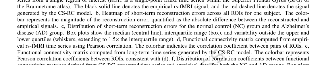Figure 3. | Lyapunov exponent analysis of reservoir computing in normal control and Alzheimer’s disease groups, are obtained from the dataset of Center 1. a,b, evolution of the first three largest Lyapunov exponents(Λ1,2,3) across iterations in the normal control (NC) group a and Alzheimer’s disease (AD) group b, with corresponding reservoir outputs shown as inset plots. c,d, the Lyapunov exponent spectra(Λk) for NC c and AD d groups, illustrating differences in stability properties. e, Distribution of the maximum Lyapunov exponents(MaxLE) calculated from n = 44 independent AD samples and n = 41 independent NC samples. Each marker denotes the group mean, with error bars representing the variability of MaxLE across subjects (reported as mean ± standard error). The blue and red colors represent the distribution of the MaxLE for the AD and NC datasets, respectively, computed using CS-RC. The green and pink colors correspond to the results obtained by estimating the MaxLE for real rs-fMRI data using Rosenstein’s method. f, showing the relationship between cognitive performance (MMSE score) and log-transformed MaxLE within the AD group(n = 44 independent AD samples). The red line represents the linear fit with a 95% confidence interval (shaded area). Spearman correlation coefficient (ρ) is 0.412, and the p-value is 0.0454, indicating a statistically significant positive correlation

Connections to Other Fields

Mathematical Skeleton

The pure mathematical core of this work involves using a specific recurrent neural network architecture, known as reservoir computing, enhanced with a compressed sensing layer for dimensionality reduction, to model and extend high-dimensional time series. From the dynamics of this learned surrogate system, fundamental invariants of nonlinear dynamics, such as Lyapunov exponents and phase synchronization values, are then compute.

Adjacent Research Areas

Nonlinear Dynamics and Chaos Theory

The calculation and interpretation of Lyapunov exponents are central to nonlinear dynamics and chaos theory. The paper uses the standard Benettin algorithm, which relies on QR decomposition to maintain the orthogonality of tangent vectors, to compute these exponents. This technique is directly borrowed from the study of chaotic systems to quantify their sensitivity to initial conditions and overall complexity. Similarly, the Phase Locking Value (PLV) is a well-established metric in nonlinear dynamics for assessing synchronization between coupled oscilators.
* A representative paper: H. Abarbanel, Analysis of Observed Chaotic Data (Springer Science & Business Media, 2012).

Echo State Networks and Machine Learning for Time Series

Reservoir computing, as employed here, is a specific and widely studied paradigm within recurrent neural networks, often referred to as Echo State Networks (ESNs). The core idea of a fixed, randomly connected "reservoir" and a trainable linear readout layer is a defining characteristic of ESNs, used for efficient learning and prediction of complex time series. The training of the output weights via ridge regression, as shown in Equation (4) ($W_{out} = UV^T(VV^T + \eta I)^{-1}$), is a standard practice in this field to prevent overfitting.
* A representative paper: H. Jaeger and H. Haas, Harnessing nonlinearity: Predicting chaotic systems and saving energy in wireless communication, Science (2004).

Sparse Signal Processing and Dimensionality Reduction

The integration of compressed sensing (CS) within the reservoir computing framework directly connects this work to sparse signal processing and dimensionality reduction. The use of a measurement matrix $\Phi$ and a sparse transform matrix $\Psi$ to reduce the dimensionality of the reservoir state $r(t)$ to $r_c(t)$ (Equation (2): $r_c(t + \Delta t) = \Phi\Psi \cdot r(t + \Delta t)$) is a direct application of CS principles. This aims to capture significant features while reducing computational burden by leveraging the inherent sparsity or compressiblity of the underlying signals.
* A representative paper: E. J. Candès and T. Tao, Near-optimal signal recovery from random projections, IEEE Transactions on Information Theory (2006).