RFWave: Multi-band Rectified Flow for Audio Waveform Reconstruction

Background & Academic Lineage

The Origin & Academic Lineage

The problem of audio waveform reconstruction, which involves generating realistic voice and sound from various compressed representations, has been a long-standing challenge in digital interactions. Its precise origin can be traced back to the fundamental need for creating perceptible sounds from low-dimensional features derived from raw audio data, enhancing user experiences in applications like virtual assistants and entertainment systems. Historically, early efforts in this academic field leveraged traditional signal processing methods, but these were soon surpassed by more advanced machine learning techniques.

The initial significant advancements came with the application of autoregressive models and Generative Adversarial Networks (GANs), as seen in pioneering works like Goodfellow et al. (2014) and Kawahara et al. (1999). These methods pushed the boundaries of audio quality beyond what was previously possible.

However, each of these earlier approaches presented its own set of "pain points" or fundamental limitations that necessitated further research, ultimately leading to papers like this one. Autoregressive models, while effective in quality, were severely hampered by their slow generation speeds. This slowness stemmed from their sequential prediction of individual sample points, making real-time applications impractical (Oord et al., 2016). GANs, on the other hand, offered faster parallel generation but struggled with issues like the complexity of discriminator designs, training instability, and the notorious problem of mode collapse (Thanh-Tung et al., 2018), where the model fails to generate a diverse range of outputs.

More recently, diffusion models emerged as a promising alternative, offering superior training stability and the ability to reconstruct high-quality waveforms (Chen et al., 2020). Yet, these models introduced a new set of limitations: they were typically an order of magnitude slower than GANs. This slowness in diffusion-based methods was primarily due to two factors: (1) the requirement for numerous sampling steps to achieve high-quality results, and (2) their operation at the individual waveform sample point level. The latter often involved multiple upsampling operations to bridge the gap from frame rate to sample rate resolution, which in turn led to higher GPU memory usage and significant computational demands. This paper, RFWave, directly addresses these limitations by aiming to match the speed of GANs while retaining the stability and quality benefits of diffusion models.

Intuitive Domain Terms

To help a zero-base reader grasp some of the specialized concepts in this paper, let's break them down with simple analogies:

• Mel-spectrograms: Imagine you're looking at a musical score, but instead of notes, it's a visual representation of how loud different sound frequencies are over time. A Mel-spectrogram is like that, but it's specifically designed to mimic how the human ear perceives sound. It emphasizes frequencies that we're more sensitive to, making it a "human-friendly" blueprint of an audio signal.
• Rectified Flow: Think of trying to move a toy car from one side of a room (noisy data) to the other (clean audio). Instead of letting the car wander around randomly or take a winding path, Rectified Flow is like having a super-smart GPS that calculates the absolute straightest, most direct route. This allows the car to reach its destination much faster and more efficiently, with fewer detours.
• Diffusion Models: Picture a very blurry photograph that gradually becomes clearer and clearer with each small adjustment. Diffusion models work similarly for audio: they start with pure, random noise (like a completely blurry sound) and, through many tiny, iterative steps, slowly "denoise" and refine it until it transforms into a clear, high-quality audio waveform.
• Short-Time Fourier Transform (STFT) frames: If you want to understand what instruments are playing in a song, you wouldn't listen to the entire song at once to figure it out. Instead, you might listen to very short snippets. STFT is like taking many quick "snapshots" of an audio signal, each showing the mix of frequencies present in that tiny moment. Processing these "snapshots" (frames) is much more manageable than dealing with the continuous, raw sound wave, making computations more efficient.

Notation Table

Here's a table of key mathematical notations used in the paper, essential for understanding the subsequent explanations:

Notation	Description

Problem Definition & Constraints

Core Problem Formulation & The Dilemma

The core problem addressed by this paper is the efficient reconstruction of high-fidelity audio waveforms from compressed representations.

The starting point (Input/Current State) for the model is either Mel-spectrograms or discrete acoustic tokens, which are compact, low-dimensional representations of audio.

The desired endpoint (Output/Goal State) is the generation of high-fidelity audio waveforms that are perceptually indistinguishable from real audio.

The exact missing link or mathematical gap this paper attempts to bridge lies in finding a generative model that can achieve both the high audio quality and training stability of diffusion models and the fast generation speeds of Generative Adversarial Networks (GANs). Mathematically, the paper leverages Rectified Flow to learn a velocity field $v(Z_t, t)$ that maps a noisy sample $Z_0$ (representing noise) to a target data distribution $Z_1$ (representing the desired audio waveform) along a straight trajectory. The objective is to minimize the deviation from this linear path:

$$ \min_v \mathbb{E}_{(X_0, X_1) \sim \gamma} \left[ \int_0^1 \left\| \frac{d}{dt} X_t - v(X_t, t) \right\|^2 dt \right] $$

where $X_t = (1-t)X_0 + tX_1$ is a simple linear interpolation between the noise and the target. The challenge is to accurately learn this velocity field with a deep neural network and then efficiently sample from it in very few steps to reconstruct complex audio.

The painful trade-off or dilemma that has trapped previous researchers is a stark choice between quality/stability and speed:
* Diffusion models (e.g., DiffWave, WaveGrad) are known for their ability to reconstruct high-quality waveforms and offer training stability. However, they are severely "hindered by latency issues due to their operation at the individual sample point level and the need for numerous sampling steps." This makes them "at least an order of magnitude slower compared to GANs," limiting their real-time applicability.
* GAN-based methods (e.g., MelGAN, HiFi-GAN) can achieve faster generation speeds by predicting sample points in parallel. Yet, they "face challenges such as the necessity for complex discriminator designs and issues like instability or mode collapse," which can compromise the quality and diversity of generated audio.

This dilemma means researchers have been forced to choose between slow, high-quality generation or fast, potentially unstable/lower-quality generation.

Constraints & Failure Modes

The problem of high-fidelity audio waveform reconstruction is insanely difficult due to several harsh, realistic constraints and their associated failure modes:

• Computational Latency & Sampling Steps: Previous diffusion models operate at the "individual sample point level" and require "numerous sampling steps" (often 50 or more) to achieve high quality. This leads to generation speeds that are "only about 10 to 20 times faster than real-time," which is insufficient for many real-world applications, especially when combined with large-scale acoustic models. The need for multiple upsampling operations to convert frame-rate features to sample-rate waveforms further increases sequence length, exacerbating computational demands.
• GPU Memory Limits: Operating at the sample point level and performing extensive upsampling results in "higher GPU memory usage." For instance, diffusion vocoders like PriorGrad, even with 30 GB of GPU memory, are limited to training on short 6-second audio clips at 44.1 kHz. This memory constraint severely restricts the length and resolution of audio that can be processed, making it a significant barrier for practical, high-resolution audio generation.
• Training Instability and Mode Collapse (GANs): GANs, while fast, are notoriously difficult to train. They require "complex discriminator designs" and are prone to "instability or mode collapse." Mode collapse means the generator might produce a limited variety of outputs, failing to capture the full diversity of the target audio distribution, leading to unnatural or repetitive sounds.
• Error Accumulation in Multi-band Processing: When audio is divided into multiple frequency subbands for processing, a common strategy, there's a risk of "error accumulation." If higher bands are conditioned on lower ones, inaccuracies in the lower bands can propagate and "adversely affect the higher bands during inference," degrading overall audio quality.
• Perceptual Artifacts from Loss Functions:
  • Standard Mean Square Error (MSE) loss, if used alone, can lead to "low-volume noise in expected silent regions." This is because small errors in quiet parts contribute minimally to the overall MSE, so the model doesn't prioritize their elimination, resulting in perceptible noise.
  • Without an "overlap loss," independently predicted subbands can exhibit "inconsistencies among them," manifesting as noticeable, abrupt transitions between frequency bands in the reconstructed audio (as visualized in Figure A.9).
  • The absence of an "STFT loss" can result in "artifacts in the presence of background noise," which might appear as vertical patterns in spectrograms (Figure A.8), reducing the perceived quality.
• Non-linear Trajectories: The effectiveness of Rectified Flow relies on learning "straight transport trajectories." If the learned velocity field deviates significantly from this ideal linear path, the numerical solvers (like the Euler method) will require more sampling steps to maintain reconstruction quality, thereby negating the speed benefits. This makes the learning of the velocity field a delicate task.
• Difficulty with High-Frequency Harmonics: Previous GAN-based methods often struggle with high-frequency components, tending to "generate horizontal lines in the high-frequency regions of the spectrograms." These artifacts are perceptually problematic, leading to a "metallic sound quality" that diminishes the naturalness of the audio, especially when applied to out-of-distribution data. This is a significant challenge for achieving truly high-fidelity audio.

Why This Approach

The Inevitability of the Choice

The adoption of Rectified Flow, coupled with a multi-band, frame-level processing strategy, was not merely an optimization but a necessary evolution to overcome fundamental limitations of existing state-of-the-art (SOTA) methods for audio waveform reconstruction. The authors recognized that while diffusion models excel at generating high-quality audio, their inherent design leads to significant latency. This slowness stems from two core issues: the need for numerous sampling steps to achieve high-fidelity outputs and their operation at the individual waveform sample point level. This sample-point-level processing drastically increases sequence length, leading to higher GPU memory usage and computational demands, making them impractical for real-time applications.

Traditional autoregressive models, despite their effectiveness, are similarly hampered by slow generation speeds due to their sequential prediction of sample points. Generative Adversarial Networks (GANs), while offering faster generation, suffer from training instability, the necessity for complex discriminator designs, and a propensity for mode collapse. Furthermore, GANs exhibit limitations in generalization and robustness, particularly when dealing with out-of-domain data, often producing artifacts like horizontal lines in high-frequency spectrogram regions.

Rectified Flow emerged as the only viable solution to bridge this gap, offering a diffusion-type model that could match GAN-based speeds while retaining the stability and high sample quality characteristic of diffusion models. The realization was that a method capable of connecting data and noise along a straight line was essential to drastically reduce the required sampling steps, thereby enhancing sampling efficiency. This, combined with a shift from sample-point to STFT frame-level operation, directly addressed the computational and memory bottlenecks that rendered prior diffusion approaches insufficient for practical, real-time audio generation.

Comparative Superiority

RFWave demonstrates qualitative superiority over previous gold standards through several structural and methodological advantages, extending beyond simple performance metrics.

Firstly, its core innovation, Rectified Flow, allows for high-quality audio generation with a drastically reduced number of sampling steps—just 10, compared to the "numerous sampling steps" required by conventional diffusion models. This is a structural advantage that directly translates to superior computational efficiency, enabling audio generation up to 160 times faster than real-time on a GPU, a speed comparable to or exceeding GANs.

Secondly, the multi-band strategy, which processes all subbands concurrently using a unified ConvNeXtV2 backbone, offers a significant structural advantage. Unlike methods that model subbands independently or condition higher bands on lower ones (which can lead to cumulative error propagation), RFWave's parallel processing not only boosts synthesis speed but also assures audio quality by circumventing these errors. This approach simplifies frequency band division by directly selecting appropriate dimensions from complex spectrograms, leading to more efficient processing and reduced error accumulation.

Thirdly, operating at the Short-Time Fourier Transform (STFT) frame level, rather than individual waveform sample points, provides a substantial memory complexity reduction. While not explicitly stated as $O(N^2)$ to $O(N)$, this frame-level processing allows RFWave to handle significantly longer audio clips (e.g., 177-second clips with the same memory resources that PriorGrad uses for 6-second clips) with greater memory efficiency. This is a critical advantage for high-resolution audio synthesis.

Qualitatively, RFWave consistently produces clearer and more consistent harmonics, especially in high-frequency ranges, leading to better overall audio quality and higher Mean Opinion Scores (MOS) compared to diffusion baselines like PriorGrad and FreGrad. For out-of-domain data, RFWave exhibits superior generalization and robustness over GAN-based models (BigVGAN, Vocos), which tend to generate perceptually problematic horizontal lines in high-frequency spectrograms, resulting in a metallic sound quality. RFWave, in contrast, maintains well-defined high-frequency harmonics, enhancing realism.

The integration of three enhanced loss functions—energy-balanced loss, overlap loss, and STFT loss—further contributes to its qualitative superiority. The energy-balanced loss mitigates low-volume noise in silent regions, a common issue with standard Mean Square Error. The overlap loss ensures smooth transitions between subbands, preventing inconsistencies. The STFT loss effectively reduces artifacts, particularly in the presence of background noise. Finally, the "equal straightness" sampling strategy, which selects time points based on the straightness of transport trajectories, ensures consistent difficulty across Euler steps and outperforms equal interval approaches in sample quality.

Alignment with Constraints

The RFWave approach perfectly aligns with the implicit constraints derived from the problem definition, which primarily revolve around achieving high-fidelity audio reconstruction with low latency, high computational efficiency, and robustness across various input types.

1. Low Latency and High Speed: The primary constraint identified for diffusion models was their slow generation speed. RFWave directly addresses this by leveraging Rectified Flow, which enables reconstruction with "just 10 sampling steps." This drastically reduces inference time, allowing RFWave to generate audio up to 160 times faster than real-time, making it practical for real-world applications where speed is paramount. The multi-band strategy further boosts synthesis speed by processing subbands concurrently.

2. High-Fidelity Audio Quality: The goal was to reconstruct "high-fidelity audio waveforms." RFWave achieves this by maintaining the training stability and high sample quality inherent to diffusion models. The incorporation of three enhanced loss functions (energy-balanced, overlap, and STFT losses) is crucial for this. The energy-balanced loss ensures accurate reconstruction even in low-volume regions, preventing perceptible noise. The overlap loss guarantees smooth transitions between subbands, avoiding artifacts. The STFT loss reduces general artifacts, especially with background noise. The "equal straightness" sampling strategy also enhances sample quality without additional computational cost.

3. Computational and Memory Efficiency: Operating at the "individual sample point level" was a major bottleneck for previous diffusion models, leading to high GPU memory usage. RFWave overcomes this by operating at the "Short-Time Fourier Transform (STFT) frame level." This frame-level processing significantly accelerates computation and reduces GPU memory usage, allowing the model to handle much longer audio clips (e.g., 177-second clips) with the same memory resources that other models use for much shorter ones. This structural choice is a direct marriage between the problem's harsh computational requirements and the solution's unique processing paradigm.

4. Versatility: The model was designed to reconstruct waveforms from "Mel-spectrograms or discrete acoustic tokens." RFWave's architecture is explicitly designed to accept both types of conditional inputs, enhancing its versatility and applicability across diverse audio generation tasks. This flexibility ensures the model is not confined to a single input representation, meeting a broad range of application needs.

Rejection of Alternatives

The paper provides clear reasoning for rejecting alternative popular approaches, highlighting their fundamental limitations in the context of high-fidelity, low-latency audio waveform reconstruction.

• Autoregressive Models: These models, such as WaveNet, were pioneering in high-quality audio generation but were rejected primarily due to their slow generation speeds. Their sequential prediction of sample points makes them computationally expensive and impractical for real-time applications, a critical constraint for RFWave.

• Generative Adversarial Networks (GANs): While GANs like HiFi-GAN and BigVGAN offer faster generation speeds, they were deemed insufficient due to inherent challenges:

  • Training Instability and Mode Collapse: GANs are notoriously difficult to train, often requiring complex discriminator designs and suffering from instability or mode collapse, which can lead to a lack of diversity in generated samples.
  • Qualitative Artifacts and Poor Generalization: Critically, GAN-based methods tend to generate "horizontal lines in the high-frequency regions of the spectrograms," which results in a "metallic sound quality" that detracts from audio naturalness. This issue is particularly pronounced when applied to out-of-domain data, where GANs show a lack of robustness and generalization compared to diffusion-type models. RFWave's ability to produce clear high-frequency harmonics even on unseen data directly addresses this failure point of GANs.

• Standard Diffusion Models (e.g., DiffWave, WaveGrad, PriorGrad, FreGrad): Despite their ability to reconstruct high-quality waveforms and offering stability during training, traditional diffusion models were rejected due to their prohibitive slowness. The paper explicitly states that these models are "at least an order of magnitude slower compared to GANs." This slowness is attributed to two key factors:

  • Numerous Sampling Steps: Standard diffusion models require a large number of iterative sampling steps to achieve high-quality outputs. Experiments showed that even with 50 sampling steps, their performance "fell short of the baseline." Rectified Flow directly tackles this by enabling high-quality generation with only 10 steps.
  • Operation at Waveform Sample Point Level: Processing audio at the individual sample point level leads to extremely long sequences, significantly increasing GPU memory usage and computational demands. RFWave's shift to STFT frame-level operation directly addresses this memory and computational bottleneck.

In essence, RFWave's design is a direct response to the shortcomings of these alternatives, aiming to combine the best aspects of diffusion (quality, stability) with the speed of GANs, while mitigating the specific issues that made each of them unsuitable for the problem's demanding requirements.

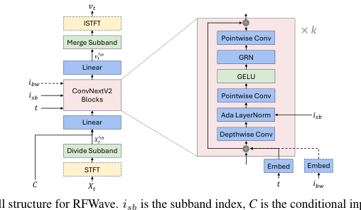Figure 1. The overall structure for RFWave. isb is the subband index, C is the conditional input, which can be an Encodec token or Mel-spectrogram, and ibw is the EnCodec bandwidth index. Modules enclosed in a dashed box, as well as dashed arrows, are considered optional

Mathematical & Logical Mechanism

The Master Equation

The RFWave model is built upon the Rectified Flow framework, which aims to learn a velocity field that transports data from a simple noise distribution to a complex data distribution along straight trajectories. The fundamental Ordinary Differential Equation (ODE) defining this flow is:

$$ \frac{dZ_t}{dt} = v(Z_t,t) \quad (1) $$

For RFWave's training, the core objective function, which incorporates an energy-balanced loss to address specific audio reconstruction challenges, is an adjusted version of the standard Rectified Flow objective. This is the primary equation that the neural network optimizes:

$$ \min E_{X_0\sim\pi_0, (X_1,C)\sim D} \left[ \int_0^1 \left\| \frac{(X_1 - X_0)}{\sigma} - \frac{v(X_t, t | C)}{\sigma} \right\|^2 dt \right] \quad (5) $$

where $X_t$ is defined by a simple linear interpolation:

$$ X_t = (1 - t)X_0 + tX_1 \quad (3) $$

Term-by-Term Autopsy

Let's dissect these equations to understand each component:

Equation (1): $\frac{dZ_t}{dt} = v(Z_t,t)$

• $Z_t$:

  • Mathematical Definition: A data point in the $d$-dimensional space $\mathbb{R}^d$ at a specific time $t$. During inference, this represents the evolving state of the audio spectrogram.
  • Physical/Logical Role: It's the "particle" or "state" that is being moved from an initial noise configuration ($Z_0$) to a target clean audio spectrogram ($Z_1$).
  • Why used: This variable tracks the trajectory of the data point through the latent space as it transforms from noise to a meaningful signal.

• $t$:

  • Mathematical Definition: A scalar time variable, typically ranging from $0$ to $1$.
  • Physical/Logical Role: Represents the progression along the trajectory. $t=0$ is the starting point (noise), and $t=1$ is the end point (target data).
  • Why used: Time is a continuous variable, and the integral over $t$ allows for modeling the continuous transformation process.

• $\frac{dZ_t}{dt}$:

  • Mathematical Definition: The instantaneous derivative of $Z_t$ with respect to time $t$. This is a vector representing the rate and direction of change of $Z_t$.
  • Physical/Logical Role: This is the "ground truth" velocity that a data point should follow to move along its trajectory. The model aims to learn this velocity.
  • Why used: It defines the ideal path. The objective function then measures how well the learned velocity field matches this ideal.

• $v(Z_t,t)$:

  • Mathematical Definition: A vector-valued function, known as the velocity field, that takes the current state $Z_t$ and time $t$ as input and outputs a velocity vector. In RFWave, this is parameterized by a deep neural network.
  • Physical/Logical Role: This is the predicted velocity field by the neural network. It dictates how $Z_t$ should move at any given time $t$. The goal of training is to make this predicted velocity match the true velocity $\frac{dZ_t}{dt}$.
  • Why used: A neural network is used because the true underlying velocity field for complex data transformations is highly non-linear and cannot be easily modeled by simple analytical functions.

Equation (5): $\min E_{X_0\sim\pi_0, (X_1,C)\sim D} \left[ \int_0^1 \left\| \frac{(X_1 - X_0)}{\sigma} - \frac{v(X_t, t | C)}{\sigma} \right\|^2 dt \right]$

• $\min$:

  • Mathematical Definition: The minimization operator.
  • Physical/Logical Role: Indicates that the training process seeks to find the parameters of the neural network $v$ that yield the smallest possible value for the entire expression.
  • Why used: This is the standard approach in machine learning to optimize model parameters by reducing a defined error metric.

• $E_{X_0\sim\pi_0, (X_1,C)\sim D}$:

  • Mathematical Definition: The expectation operator, averaging the loss over samples drawn from the specified distributions.
  • Physical/Logical Role: Ensures that the learned velocity field generalizes well across the entire distribution of possible noise inputs ($X_0$) and target data-condition pairs ($(X_1, C)$).
  • Why used: Training on individual samples would lead to overfitting. Taking an expectation over the data distributions allows the model to learn a robust, generalizable velocity field.

• $X_0$:

  • Mathematical Definition: An initial data point sampled from a simple distribution $\pi_0$, typically standard Gaussian noise.
  • Physical/Logical Role: Represents the starting point of the generation process, a "blank canvas" of noise that will be transformed into an audio spectrogram.
  • Why used: Gaussian noise is a common, easy-to-sample distribution, providing a consistent starting point for the flow.

• $\pi_0$:

  • Mathematical Definition: The probability distribution of the initial noise states.
  • Physical/Logical Role: Defines the characteristics of the noise from which the generation process begins.
  • Why used: A simple, well-understood distribution like Gaussian noise simplifies the initial state and provides a clear reference for the start of the flow.

• $X_1$:

  • Mathematical Definition: A target data point (clean audio spectrogram) sampled from the dataset $D$.
  • Physical/Logical Role: Represents the desired output, the "ground truth" audio spectrogram that the model aims to reconstruct.
  • Why used: This is the ultimate destination of the Rectified Flow trajectory, providing the target for the transformation.

• $C$:

  • Mathematical Definition: Conditional information, such as Mel-spectrograms or discrete acoustic tokens, associated with $X_1$.
  • Physical/Logical Role: Guides the generation process, telling the model what kind of audio spectrogram to produce. For example, if $C$ is a Mel-spectrogram, the model should generate a waveform matching that spectrogram.
  • Why used: This allows for conditional generation, where the output is controlled by an input condition, making the model useful for tasks like vocoding.

• $D$:

  • Mathematical Definition: The empirical dataset distribution of paired $(X_1, C)$ samples.
  • Physical/Logical Role: Represents the real-world data that the model learns from.
  • Why used: The model learns to generate realistic data by observing and matching the patterns present in this dataset.

• $X_t$:

  • Mathematical Definition: An interpolated data point at time $t$, calculated as $X_t = (1 - t)X_0 + tX_1$.
  • Physical/Logical Role: Represents an intermediate state along a straight line path between $X_0$ and $X_1$. This linear path defines the "ground truth" trajectory that the Rectified Flow aims to mimic.
  • Why used: The linear interpolation simplifies the "true" velocity calculation to $(X_1 - X_0)$, making the learning task easier for the neural network to approximate a constant velocity field.

• $\sigma$:

  • Mathematical Definition: The standard deviation of the difference $(X_1 - X_0)$. It's calculated as $\sqrt{\text{Var}_t(X_1 - X_0)}$ along the feature dimension for each frequency subband.
  • Physical/Logical Role: Acts as a weighting factor in the energy-balanced loss. By dividing both the true and predicted velocities by $\sigma$, the loss emphasizes errors in regions where the signal difference $(X_1 - X_0)$ has low variance (e.g., silent regions). This prevents the model from ignoring small errors in quiet parts of the audio.
  • Why used: The paper notes that standard MSE (without $\sigma$) tends to overlook small errors in low-volume regions. Normalizing by $\sigma$ balances the contribution of errors across different energy levels, ensuring high-quality reconstruction even in silent or low-amplitude segments. This is a key innovation for audio quality.

• $v(X_t, t | C)$:

  • Mathematical Definition: The velocity field predicted by the neural network, conditioned on $C$, at the interpolated state $X_t$ and time $t$.
  • Physical/Logical Role: This is the model's best guess for the velocity required to move from $X_0$ to $X_1$ at time $t$, given the condition $C$.
  • Why used: It's the output of the neural network that is being trained to match the target velocity.

• $\left\| \cdot \right\|^2$:

  • Mathematical Definition: The squared L2 norm (Euclidean distance). For vectors $a$ and $b$, $||a - b||^2 = \sum (a_i - b_i)^2$.
  • Physical/Logical Role: Measures the squared difference (error) between the normalized true velocity and the normalized predicted velocity. Squaring penalizes larger errors more heavily.
  • Why used: The L2 norm is a common and differentiable loss function, suitable for gradient-based optimization. It quantifies the "distance" between the model's prediction and the target.

• $\int_0^1 \cdot dt$:

  • Mathematical Definition: A definite integral over the time interval $[0, 1]$.
  • Physical/Logical Role: Averages the squared error across the entire trajectory from $t=0$ to $t=1$. This ensures that the velocity field is accurate at all points along the path, not just at specific times.
  • Why used: The transformation is continuous in time, so integrating over the entire time interval provides a comprehensive measure of error for the continuous flow. It's approximated by a summation over discrete time steps during training.

Step-by-Step Flow

Imagine a single abstract data point, representing an audio spectrogram, moving through the RFWave system.

During Training (Learning the Velocity Field):

1. Initialization: For each training step, the system first samples a pair of data points:

   • A random noise vector $X_0$ is drawn from a simple Gaussian distribution ($\pi_0$). This is our starting "blank canvas."
   • A clean target audio spectrogram $X_1$ and its corresponding conditional information $C$ (e.g., a Mel-spectrogram) are sampled from the real-world dataset $D$. This is our desired final output.

2. Trajectory Definition: The system then defines a straight line path between $X_0$ and $X_1$. For any given time $t$ between 0 and 1, an intermediate point $X_t$ is calculated using linear interpolation: $X_t = (1 - t)X_0 + tX_1$. This means the "true" velocity required to travel this straight path is simply $X_1 - X_0$.

3. Energy Balancing: To prevent the model from ignoring subtle details in quieter audio regions, the true velocity $(X_1 - X_0)$ is normalized by $\sigma$, the standard deviation of $(X_1 - X_0)$ along the feature dimension. This re-weights the importance of errors across different energy levels.

4. Velocity Prediction: The neural network, which represents the velocity field $v$, takes the current interpolated state $X_t$, the time $t$, and the conditional input $C$ as its inputs. It then outputs its prediction for the velocity vector $v(X_t, t | C)$ that should be applied to $X_t$. This predicted velocity is also normalized by $\sigma$.

5. Error Calculation: The system calculates the squared L2 norm of the difference between the normalized true velocity and the normalized predicted velocity. This difference represents how far off the model's predicted movement is from the ideal straight-line movement. This error is computed for many discrete time steps between $t=0$ and $t=1$ and then summed up (approximating the integral).

6. Model Update: This accumulated error (the loss) is then used to update the neural network's parameters via backpropagation and an optimizer (like AdamW). The network adjusts its internal weights and biases to reduce this error, effectively learning to predict velocities that guide $X_0$ towards $X_1$ along straighter, more accurate paths.

During Inference (Generating Audio):

1. Initial Noise: The process begins by sampling an initial noise vector $Z_0$ from the Gaussian distribution. This is the starting point for the generation.

2. Iterative Transformation: The model then iteratively transforms $Z_t$ over a small number of discrete time steps (e.g., 10 steps) using a numerical solver like Euler's method. For each step $i$ from $0$ to $N-1$:

   • Time Step Calculation: A small time interval $dt = t_{i+1} - t_i$ is determined. (The paper proposes an "equal straightness" method for selecting these $t_i$ points, which is more sophisticated than equal intervals).
   • Domain Conversion (if time domain): If the model operates in the time domain, the current state $Z_{t_i}$ is first converted to the frequency domain using a Short-Time Fourier Transform (STFT). This is because the neural network operates at the STFT frame level.
   • Velocity Prediction: The neural network $v$ takes the current (potentially frequency-domain) state $Z_{t_i}$, the current time $t_i$, and the conditional input $C$ (e.g., Mel-spectrogram) to predict the velocity $v(Z_{t_i}, t_i | C)$.
   • Domain Conversion (if time domain): If the model operates in the time domain, the predicted velocity $v$ is converted back to the time domain using an Inverse Short-Time Fourier Transform (ISTFT).
   • State Update: The current state $Z_{t_i}$ is updated to the next state $Z_{t_{i+1}}$ by adding the predicted velocity multiplied by the time step: $Z_{t_{i+1}} = Z_{t_i} + v(Z_{t_i}, t_i | C) \cdot dt$. This is like taking a small step in the direction of the predicted velocity.

3. Final Output: After $N$ steps, the final state $Z_N$ is obtained. This $Z_N$ is the reconstructed audio spectrogram.

4. Domain Conversion (if frequency domain): If the model operated entirely in the frequency domain during inference, a single ISTFT is applied to $Z_N$ to convert it into the final audio waveform in the time domain.

This process transforms the initial noise into a high-fidelity audio waveform, guided by the learned velocity field and the provided conditional information.

Optimization Dynamics

The RFWave model learns and converges by iteratively refining its neural network's ability to predict the "straightest" possible velocity field. Here's how the optimization dynamics play out:

1. Loss Landscape Shaping: The core of RFWave's learning is minimizing the energy-balanced loss (Equation 5). This loss function is critical in shaping the optimization landscape. Unlike a standard Mean Squared Error (MSE) that might prioritize reducing errors in high-amplitude regions, the division by $\sigma$ (the standard deviation of $X_1 - X_0$) re-weights the errors. This means that errors in low-volume or silent regions, where $\sigma$ would be small, are given proportionally more importance. This effectively flattens the loss landscape in high-amplitude areas and steepens it in low-amplitude areas, forcing the model to pay close attention to subtle noise and artifacts that would otherwise be perceptually noticeable. This is a clever trick to improve audio quality.

2. Gradient Behavior: During training, the AdamW optimizer computes gradients of the loss function with respect to the neural network's parameters. These gradients indicate the direction and magnitude of parameter adjustments needed to reduce the loss. Because of the $\sigma$ normalization, gradients arising from errors in quiet sections will be relatively larger than they would be with standard MSE, ensuring that the model actively learns to suppress low-volume noise. The goal is to drive these gradients towards zero, indicating that the predicted velocity field $v(X_t, t | C)$ closely matches the ideal straight-line velocity $(X_1 - X_0)$.

3. Iterative State Updates (Parameter Learning): The neural network's parameters are updated iteratively based on these gradients. Each update pushes the model towards a state where its predicted velocity field more accurately guides the transformation from noise ($X_0$) to target ($X_1$) along linear trajectories. The ConvNeXtV2 backbone, with its deep convolutional structure, is adept at capturing complex patterns in spectrograms and learning this intricate velocity mapping.

4. Straightness and Sampling Efficiency: The Rectified Flow framework inherently encourages straight trajectories. When the learned velocity field $v(X_t, t | C)$ perfectly matches $(X_1 - X_0)$, the trajectories are perfectly straight. This straightness is crucial for fast inference because it allows the model to use a very small number of sampling steps (e.g., 10 steps) with numerical solvers like Euler's method, without significant loss of quality. If the trajectories were highly curved, many more steps would be needed to accurately follow the path, slowing down inference.

5. Equal Straightness Sampling Strategy: RFWave further refines its optimization and convergence by employing an "equal straightness" sampling strategy for selecting time points during inference (and implicitly influencing training). Instead of using equally spaced time intervals, this strategy selects time points such that the increase in straightness is consistent across each interval. This means that if a particular segment of the trajectory is inherently less straight (i.e., the model's current $v$ deviates more from $(X_1 - X_0)$), more sampling steps will be allocated to that region. This adaptive allocation of computational effort during inference effectively smooths out the "difficulty" of each Euler step, leading to better sample quality for a fixed number of steps. It also implicitly guides the training to improve the velocity field in these "harder" regions.

In essence, RFWave's optimization dynamics are a sophisticated interplay of a carefully designed loss function that shapes the error landscape, gradient-based parameter updates, and an intelligent sampling strategy that together ensure the model learns to generate high-quality audio efficiently by maintaining straight, energy-balanced trajectories.

Results, Limitations & Conclusion

Experimental Design & Baselines

The authors meticulously designed their experiments to rigorously validate RFWave's performance, employing both objective metrics and subjective human evaluations. For Mel-spectrogram inputs, RFWave was benchmarked against two categories of "victims": state-of-the-art diffusion vocoders and widely-used GAN-based models. The diffusion baselines included PriorGrad and FreGrad, while the GAN baselines were BigVGAN and Vocos. For discrete EnCodec token inputs, RFWave was compared against EnCodec itself and Multi-Band Diffusion (MBD).

To ensure a comprehensive comparison, models were trained on diverse datasets covering various audio categories. For Mel-spectrogram inputs, separate RFWave models were trained on LibriTTS (speech), MTG-Jamendo (music), and Opencpop (vocal) datasets. In-domain performance against GANs was assessed on LibriTTS, while out-of-domain generalization was tested on the MUSDB18 dataset. For discrete EnCodec tokens, a universal RFWave model was trained on a large-scale mixed dataset comprising Common Voice 7.0, DNS Challenge 4, MTG-Jamendo, FSD50K, and AudioSet, and evaluated on a unified test set of 900 samples from 15 external datasets.

The experimental setup for baselines followed their authors' recommendations: PriorGrad used 6 sampling steps, FreGrad 50, and MBD 20. In contrast, RFWave consistently used only 10 sampling steps. Objective evaluation relied on standard metrics: ViSQOL for perceptual quality, PESQ for speech quality, V/UV F1 for voiced/unvoiced classification, and Periodicity error. Subjective evaluation involved crowd-sourced assessments using a 5-point Mean Opinion Score (MOS) scale, where 30 listeners rated audio naturalness. The default RFWave configuration for evaluation utilized a time-domain model with three enhanced loss functions (energy-balanced, overlap, and STFT loss), an 8-layer ConvNeXtV2 backbone, and 8 equally spanned subbands. All inference speed benchmarks were conducted on an NVIDIA GeForce RTX 4090 GPU.

What the Evidence Proves

The empirical evidence overwhelmingly demonstrates RFWave's superior performance, particularly in terms of reconstruction quality and computational efficiency.

Against diffusion-based models (PriorGrad and FreGrad), RFWave consistently achieved higher MOS, PESQ, ViSQOL, and V/UV F1 scores, alongside lower Periodicity error across all tested datasets (LibriTTS, MTG-Jamendo, Opencpop). For instance, on average across various test sets, RFWave achieved a MOS of 3.95 compared to PriorGrad's 3.75 and FreGrad's 2.99 (Table 1). The definitive evidence for its core mechanism's effectiveness lies in its ability to produce "clearer and more consistent harmonics, particularly in high-frequency ranges," which was visually confirmed through spectrogram comparisons (Figures A.3, A.4, A.5). These figures clearly show RFWave generating clean and stable harmonics, while baselines exhibited minor discontinuities or blurred high-frequency components. This directly validates the Rectified Flow's straight transport trajectories and the multi-band, frame-level processing.

When pitted against GAN-based models (BigVGAN and Vocos) on in-domain data (LibriTTS), RFWave performed comparably (e.g., MOS 3.82 for RFWave vs. 3.78 for BigVGAN, Table 2). However, its true strength emerged in out-of-domain generalization on the MUSDB18 dataset, where RFWave showed significant advantages in MOS (e.g., average MOS 3.67 for RFWave vs. 3.51 for BigVGAN, Table 3). The paper highlights that GAN-based methods tend to generate "horizontal lines in the high-frequency regions of the spectrograms," leading to a "metallic sound quality." In contrast, RFWave consistently produced "clear high-frequency harmonics" even on out-of-domain data (Figure A.7), proving its robustness and generalization capabilities, a key advantage of diffusion-type models.

For discrete EnCodec token inputs, RFWave (with Classifier-Free Guidance) achieved optimal scores in most objective and subjective metrics across various bandwidths (1.5, 3.0, 6.0, 12.0 kbps) when compared to EnCodec and MBD (Table 4). For example, at 6.0 kbps, RFWave's MOS was 3.69, significantly higher than EnCodec's 3.10 and MBD's 3.43. While ViSQOL showed a slight bias towards EnCodec's GAN-based decoder, RFWave's overall performance was superior.

Ablation studies provided crucial insights into the efficacy of individual components. The time-domain model consistently outperformed its frequency-domain counterpart, particularly in preserving high-frequency details (Table 5). The Rectified Flow mechanism itself was shown to be critical, as a DDPM approach with 50 sampling steps performed poorly compared to RFWave's 10 steps (Table 6). The ConvNeXtV2 backbone also proved superior to a ResNet backbone, enhancing both efficiency and audio quality. Each of the three enhanced loss functions contributed positively: the energy-balanced loss mitigated low-volume noise, the overlap loss ensured smooth subband transitions (Figure A.9), and the STFT loss reduced artifacts (Figure A.8). Crucially, the "equal straightness" time point selection method consistently outperformed the equal interval approach, enhancing sample quality "for free."

Finally, RFWave demonstrated vastly superior computational efficiency. It achieved audio generation speeds up to 160 times faster than real-time on a GPU (162.59 xRT), making it the fastest diffusion-based audio waveform reconstruction model to date. It was more than twice as fast as BigVGAN (72.68 xRT) and consumed less GPU memory (780 MB vs 1436 MB), effectively eliminating latency as a barrier for practical applications (Table 7). This speed advantage is even more pronounced for high-resolution audio, underscoring the benefit of its frame-level, multi-band operation.

Limitations & Future Directions

While RFWave presents a significant leap forward in audio waveform reconstruction, the paper also implicitly highlights a few areas that warrant further consideration and development.

One notable observation is the subtle bias of the ViSQOL metric towards GAN-based models, where EnCodec's GAN-based decoder sometimes excelled despite RFWave's overall superior performance. This suggests that while RFWave produces perceptually high-quality audio, there might be specific waveform characteristics that ViSQOL is tuned to, which RFWave doesn't fully capture. This isn't a limitation of RFWave's quality per se, but rather a challenge in how we objectively measure and compare audio synthesis.

Another interesting trade-off was observed with the STFT loss: while it effectively reduced artifacts and improved PESQ, it sometimes degraded ViSQOL and periodicity scores. This indicates a tension between different aspects of audio quality, where optimizing for one might come at the expense of another. The time-domain model, while achieving slightly better performance, also requires STFT and ISTFT operations at each sampling step, which introduces computational overhead compared to the frequency-domain approach that only needs a single ISTFT at the end. Although the authors state their experiments show the time-domain configuration performs better despite this, it's still an added complexity. Lastly, the Classifier-Free Guidance (CFG) showed little improvement for Mel-spectrogram inputs, suggesting its effectiveness might be context-dependent, primarily benefiting more compressed inputs like EnCodec tokens.

Looking ahead, several exciting discussion topics emerge from these findings:

• Perceptual Metric Development: Given the ViSQOL bias and the STFT loss trade-off, how can we develop more comprehensive and perceptually aligned objective metrics that capture the nuances of audio quality without favoring specific model architectures? This could involve incorporating human auditory system models or learning perceptual distances.
• Adaptive Loss Weighting: The current loss functions (energy-balanced, overlap, STFT) have fixed weights. Future research could explore dynamic or adaptive weighting schemes for these losses, perhaps based on the input audio characteristics or the current training stage, to achieve a more balanced optimization across various quality dimensions.
• Real-time Deployment on Edge Devices: While 160x real-time on a high-end GPU is impressive, the next frontier is efficient deployment on more constrained hardware, such as mobile devices or embedded systems. This would involve exploring model quantization, pruning, or specialized hardware accelerators to maintain high quality and speed with limited resources.
• Beyond Rectified Flow: Rectified Flow is a powerful mechanism for straight trajectories. Could advancements in other flow-matching techniques or novel ODE solvers further reduce the required sampling steps, potentially pushing inference speeds even higher or enabling even more complex audio generation tasks?
• Dynamic Sampling Strategies: The "equal straightness" time point selection is calculated once. Could an adaptive sampling strategy, where time points are dynamically adjusted during inference based on the current state of the audio generation, lead to further improvements in quality or efficiency for particularly challenging audio segments?
• Multimodal Integration and Control: RFWave reconstructs from Mel-spectrograms or discrete acoustic tokens. How can this robust vocoder be seamlessly integrated into larger multimodal generative systems, such as text-to-audio, video-to-audio, or even interactive music synthesis, allowing for fine-grained control over various audio attributes beyond just waveform reconstruction?
• Understanding High-Frequency Harmonics: The paper highlights RFWave's ability to generate "clear high-frequency harmonics" compared to GANs' "horizontal lines." A deeper theoretical and empirical investigation into why Rectified Flows excel at this specific aspect could lead to new insights for designing future audio generative models. This could involve analyzing the spectral properties of the learned velocity fields.

Connections to Other Fields

Mathematical Skeleton

The pure mathematical core of this work lies in learning a velocity field $v(Z_t, t)$ that defines an Ordinary Differential Equation (ODE) $dZ_t/dt = v(Z_t, t)$, which transports samples from an initial noise distribution $X_0$ to a target data distribution $X_1$ along approximately straight trajectories $X_t = (1-t)X_0 + tX_1$. The learning objective minimizes the deviation of the learned velocity field from these linear paths, effectively performing a form of flow matching.

Adjacent Research Areas

Optimal Transport

Rectified Flow, as employed in this paper, is deeply connected to the field of Optimal Transport (OT). The fundamental goal of finding a "straight" or "minimal cost" path between two probability distributions is central to both. Specifically, the objective function in Equation 2, $\min_v E_{(X_0, X_1)\sim\gamma} \int_0^1 || \frac{d}{dt} X_t - v(X_t, t) ||^2 dt$, where $X_t = (1-t)X_0 + tX_1$, is a direct formulation of a flow matching problem. This seeks to learn a vector field $v$ that pushes forward samples from one distribution to another along paths that are as linear as possible, which can be seen as a relaxation or approximation of finding an optimal transport map, particularly in the context of the 2-Wasserstein distance. The straightness of the trajectories is a key characteristic that distinguishes Rectified Flow from more general continuous flows, aiming for computational efficiency in transport. For a comprehensive overview of the underlying theory, one might refer to works like Villani (2009) on optimal transport theory, or the foundational papers on Rectified Flow itself, such as Liu et al. (2023) and Lipman et al. (2023), which explicitly link it to OT.

Diffusion Models / Score-based Generative Models

This work presents RFWave as a "diffusion-type" model, highlighting its strong ties to the broader family of diffusion and score-based generative models. While traditional diffusion models often learn a score function or a noise prediction network, Rectified Flow learns a velocity field $v(Z_t, t)$ that governs a deterministic ODE. This ODE is analagous to the probability flow ODE found in score-based generative models (Song et al., 2020) or the reverse ODE in denoising diffusion probabilistic models (Ho et al., 2020) when the noise schedule is simplified. Both paradigms define a continuous-time process to transform a simple noise distribution into a complex data distribution. The sampling process in RFWave, using an Euler method to solve the ODE, directly mirrors the reverse sampling steps in diffusion models, albeit with a focus on achieving high quality with fewer steps due to the straight trajectories.

Neural Ordinary Differential Equations (Neural ODEs)

The mathematical structure of Rectified Flow, $dZ_t/dt = v(Z_t, t)$ where $v$ is parameterized by a deep neural network, places it squarely within the domain of Neural Ordinary Differential Equations. Neural ODEs define continuous transformations by learning the dynamics of an ODE using a neural network. In this paper, the neural network learns the velocity field that dictates how samples evolve over time from noise to data. This approach allows for flexible and continuous transformations, and the "equal straightness" sampling strategy (Section 3.3) is an optimization technique for numerically integrating this learned ODE more efficiently. The ability to model complex transformations via continuous dynamics, where the neural network defines the instantaneous rate of change, is a core concept shared with general Neural ODEs (Chen et al., 2018), which are often used in continuous normalizing flows for density estimation and generative tasks. The paper's use of a ConvNeXtV2 backbone to model $v$ is a practical application of this principle, allowing the network to learn intricate temporal and spectral dynamics.

Mathematical & Logical Mechanism

The Master Equation

The RFWave model is built upon the Rectified Flow framework, which aims to learn a velocity field that transports data from a simple noise distribution to a complex data distribution along straight trajectories. The fundamental Ordinary Differential Equation (ODE) defining this flow is:

$$ \frac{dZ_t}{dt} = v(Z_t,t) \quad (1) $$

For RFWave's training, the core objective function, which incorporates an energy-balanced loss to address specific audio reconstruction challenges, is an adjusted version of the standard Rectified Flow objective. This is the primary equation that the neural network optimizes:

$$ \min E_{X_0\sim\pi_0, (X_1,C)\sim D} \left[ \int_0^1 \left\| \frac{(X_1 - X_0)}{\sigma} - \frac{v(X_t, t | C)}{\sigma} \right\|^2 dt \right] \quad (5) $$

where $X_t$ is defined by a simple linear interpolation:

$$ X_t = (1 - t)X_0 + tX_1 \quad (3) $$

Term-by-Term Autopsy

Let's dissect these equations to understand each component:

Equation (1): $\frac{dZ_t}{dt} = v(Z_t,t)$

• $Z_t$:

  • Mathematical Definition: A data point in the $d$-dimensional space $\mathbb{R}^d$ at a specific time $t$. During inference, this represents the evolving state of the audio spectrogram.
  • Physical/Logical Role: It's the "particle" or "state" that is being moved from an initial noise configuration ($Z_0$) to a target clean audio spectrogram ($Z_1$).
  • Why used: This variable tracks the trajectory of the data point through the latent space as it transforms from noise to a meaningful signal.

• $t$:

  • Mathematical Definition: A scalar time variable, typically ranging from $0$ to $1$.
  • Physical/Logical Role: Represents the progression along the trajectory. $t=0$ is the starting point (noise), and $t=1$ is the end point (target data).
  • Why used: Time is a continuous variable, and the integral over $t$ allows for modeling the continuous transformation process.

• $\frac{dZ_t}{dt}$:

  • Mathematical Definition: The instantaneous derivative of $Z_t$ with respect to time $t$. This is a vector representing the rate and direction of change of $Z_t$.
  • Physical/Logical Role: This is the "ground truth" velocity that a data point should follow to move along its trajectory. The model aims to learn this velocity.
  • Why used: It defines the ideal path. The objective function then measures how well the learned velocity field matches this ideal.

• $v(Z_t,t)$:

  • Mathematical Definition: A vector-valued function, known as the velocity field, that takes the current state $Z_t$ and time $t$ as input and outputs a velocity vector. In RFWave, this is parameterized by a deep neural network.
  • Physical/Logical Role: This is the predicted velocity field by the neural network. It dictates how $Z_t$ should move at any given time $t$. The goal of training is to make this predicted velocity match the true velocity $\frac{dZ_t}{dt}$.
  • Why used: A neural network is used because the true underlying velocity field for complex data transformations is highly non-linear and cannot be easily modeled by simple analytical functions.

Equation (5): $\min E_{X_0\sim\pi_0, (X_1,C)\sim D} \left[ \int_0^1 \left\| \frac{(X_1 - X_0)}{\sigma} - \frac{v(X_t, t | C)}{\sigma} \right\|^2 dt \right]$

• $\min$:

  • Mathematical Definition: The minimization operator.
  • Physical/Logical Role: Indicates that the training process seeks to find the parameters of the neural network $v$ that yield the smallest possible value for the entire expression.
  • Why used: This is the standard approach in machine learning to optimize model parameters by reducing a defined error metric.

• $E_{X_0\sim\pi_0, (X_1,C)\sim D}$:

  • Mathematical Definition: The expectation operator, averaging the loss over samples drawn from the specified distributions.
  • Physical/Logical Role: Ensures that the learned velocity field generalizes well across the entire distribution of possible noise inputs ($X_0$) and target data-condition pairs ($(X_1, C)$).
  • Why used: Training on individual samples would lead to overfitting. Taking an expectation over the data distributions allows the model to learn a robust, generalizable velocity field.

• $X_0$:

  • Mathematical Definition: An initial data point sampled from a simple distribution $\pi_0$, typically standard Gaussian noise.
  • Physical/Logical Role: Represents the starting point of the generation process, a "blank canvas" of noise that will be transformed into an audio spectrogram.
  • Why used: Gaussian noise is a common, easy-to-sample distribution, providing a consistent starting point for the flow.

• $\pi_0$:

  • Mathematical Definition: The probability distribution of the initial noise states.
  • Physical/Logical Role: Defines the characteristics of the noise from which the generation process begins.
  • Why used: A simple, well-understood distribution like Gaussian noise simplifies the initial state and provides a clear reference for the start of the flow.

• $X_1$:

  • Mathematical Definition: A target data point (clean audio spectrogram) sampled from the dataset $D$.
  • Physical/Logical Role: Represents the desired output, the "ground truth" audio spectrogram that the model aims to reconstruct.
  • Why used: This is the ultimate destination of the Rectified Flow trajectory, providing the target for the transformation.

• $C$:

  • Mathematical Definition: Conditional information, such as Mel-spectrograms or discrete acoustic tokens, associated with $X_1$.
  • Physical/Logical Role: Guides the generation process, telling the model what kind of audio spectrogram to produce. For example, if $C$ is a Mel-spectrogram, the model should generate a waveform matching that spectrogram.
  • Why used: This allows for conditional generation, where the output is controlled by an input condition, making the model useful for tasks like vocoding.

• $D$:

  • Mathematical Definition: The empirical dataset distribution of paired $(X_1, C)$ samples.
  • Physical/Logical Role: Represents the real-world data that the model learns from.
  • Why used: The model learns to generate realistic data by observing and matching the patterns present in this dataset.

• $X_t$:

  • Mathematical Definition: An interpolated data point at time $t$, calculated as $X_t = (1 - t)X_0 + tX_1$.
  • Physical/Logical Role: Represents an intermediate state along a straight line path between $X_0$ and $X_1$. This linear path defines the "ground truth" trajectory that the Rectified Flow aims to mimic.
  • Why used: The linear interpolation simplifies the "true" velocity calculation to $(X_1 - X_0)$, making the learning task easier for the neural network to approximate a constant velocity field.

• $\sigma$:

  • Mathematical Definition: The standard deviation of the difference $(X_1 - X_0)$. It's calculated as $\sqrt{\text{Var}_t(X_1 - X_0)}$ along the feature dimension for each frequency subband.
  • Physical/Logical Role: Acts as a weighting factor in the energy-balanced loss. By dividing both the true and predicted velocities by $\sigma$, the loss emphasizes errors in regions where the signal difference $(X_1 - X_0)$ has low variance (e.g., silent regions). This prevents the model from ignoring small errors in quiet parts of the audio.
  • Why used: The paper notes that standard MSE (without $\sigma$) tends to overlook small errors in low-volume regions. Normalizing by $\sigma$ balances the contribution of errors across different energy levels, ensuring high-quality reconstruction even in silent or low-amplitude segments. This is a key innovation for audio quality.

• $v(X_t, t | C)$:

  • Mathematical Definition: The velocity field predicted by the neural network, conditioned on $C$, at the interpolated state $X_t$ and time $t$.
  • Physical/Logical Role: This is the model's best guess for the velocity required to move from $X_0$ to $X_1$ at time $t$, given the condition $C$.
  • Why used: It's the output of the neural network that is being trained to match the target velocity.

• $\left\| \cdot \right\|^2$:

  • Mathematical Definition: The squared L2 norm (Euclidean distance). For vectors $a$ and $b$, $||a - b||^2 = \sum (a_i - b_i)^2$.
  • Physical/Logical Role: Measures the squared difference (error) between the normalized true velocity and the normalized predicted velocity. Squaring penalizes larger errors more heavily.
  • Why used: The L2 norm is a common and differentiable loss function, suitable for gradient-based optimization. It quantifies the "distance" between the model's prediction and the target.

• $\int_0^1 \cdot dt$:

  • Mathematical Definition: A definite integral over the time interval $[0, 1]$.
  • Physical/Logical Role: Averages the squared error across the entire trajectory from $t=0$ to $t=1$. This ensures that the velocity field is accurate at all points along the path, not just at specific times.
  • Why used: The transformation is continuous in time, so integrating over the entire time interval provides a comprehensive measure of error for the continuous flow. It's approximated by a summation over discrete time steps during training.

Step-by-Step Flow

Imagine a single abstract data point, representing an audio spectrogram, moving through the RFWave system.

During Training (Learning the Velocity Field):

1. Initialization: For each training step, the system first samples a pair of data points:

   • A random noise vector $X_0$ is drawn from a simple Gaussian distribution ($\pi_0$). This is our starting "blank canvas."
   • A clean target audio spectrogram $X_1$ and its corresponding conditional information $C$ (e.g., a Mel-spectrogram) are sampled from the real-world dataset $D$. This is our desired final output.

2. Trajectory Definition: The system then defines a straight line path between $X_0$ and $X_1$. For any given time $t$ between 0 and 1, an intermediate point $X_t$ is calculated using linear interpolation: $X_t = (1 - t)X_0 + tX_1$. This means the "true" velocity required to travel this straight path is simply $X_1 - X_0$.

3. Energy Balancing: To prevent the model from ignoring subtle details in quieter audio regions, the true velocity $(X_1 - X_0)$ is normalized by $\sigma$, the standard deviation of $(X_1 - X_0)$ along the feature dimension. This re-weights the importance of errors across different energy levels.

4. Velocity Prediction: The neural network, which represents the velocity field $v$, takes the current interpolated state $X_t$, the time $t$, and the conditional input $C$ as its inputs. It then outputs its prediction for the velocity vector $v(X_t, t | C)$ that should be applied to $X_t$. This predicted velocity is also normalized by $\sigma$.

5. Error Calculation: The system calculates the squared L2 norm of the difference between the normalized true velocity and the normalized predicted velocity. This difference represents how far off the model's predicted movement is from the ideal straight-line movement. This error is computed for many discrete time steps between $t=0$ and $t=1$ and then summed up (approximating the integral).

6. Model Update: This accumulated error (the loss) is then used to update the neural network's parameters via backpropagation and an optimizer (like AdamW). The network adjusts its internal weights and biases to reduce this error, effectively learning to predict velocities that guide $X_0$ towards $X_1$ along straighter, more accurate paths.

During Inference (Generating Audio):

1. Initial Noise: The process begins by sampling an initial noise vector $Z_0$ from the Gaussian distribution. This is the starting point for the generation.

2. Iterative Transformation: The model then iteratively transforms $Z_t$ over a small number of discrete time steps (e.g., 10 steps) using a numerical solver like Euler's method. For each step $i$ from $0$ to $N-1$:

   • Time Step Calculation: A small time interval $dt = t_{i+1} - t_i$ is determined. (The paper proposes an "equal straightness" method for selecting these $t_i$ points, which is more sophisticated than equal intervals).
   • Domain Conversion (if time domain): If the model operates in the time domain, the current state $Z_{t_i}$ is first converted to the frequency domain using a Short-Time Fourier Transform (STFT). This is because the neural network operates at the STFT frame level.
   • Velocity Prediction: The neural network $v$ takes the current (potentially frequency-domain) state $Z_{t_i}$, the current time $t_i$, and the conditional input $C$ (e.g., Mel-spectrogram) to predict the velocity $v(Z_{t_i}, t_i | C)$.
   • Domain Conversion (if time domain): If the model operates in the time domain, the predicted velocity $v$ is converted back to the time domain using an Inverse Short-Time Fourier Transform (ISTFT).
   • State Update: The current state $Z_{t_i}$ is updated to the next state $Z_{t_{i+1}}$ by adding the predicted velocity multiplied by the time step: $Z_{t_{i+1}} = Z_{t_i} + v(Z_{t_i}, t_i | C) \cdot dt$. This is like taking a small step in the direction of the predicted velocity.

3. Final Output: After $N$ steps, the final state $Z_N$ is obtained. This $Z_N$ is the reconstructed audio spectrogram.

4. Domain Conversion (if frequency domain): If the model operated entirely in the frequency domain during inference, a single ISTFT is applied to $Z_N$ to convert it into the final audio waveform in the time domain.

This process transforms the initial noise into a high-fidelity audio waveform, guided by the learned velocity field and the provided conditional information.

Optimization Dynamics

The RFWave model learns and converges by iteratively refining its neural network's ability to predict the "straightest" possible velocity field. Here's how the optimization dynamics play out:

1. Loss Landscape Shaping: The core of RFWave's learning is minimizing the energy-balanced loss (Equation 5). This loss function is critical in shaping the optimization landscape. Unlike a standard Mean Squared Error (MSE) that might prioritize reducing errors in high-amplitude regions, the division by $\sigma$ (the standard deviation of $X_1 - X_0$) re-weights the errors. This means that errors in low-volume or silent regions, where $\sigma$ would be small, are given proportionally more importance. This effectively flattens the loss landscape in high-amplitude areas and steepens it in low-amplitude areas, forcing the model to pay close attention to subtle noise and artifacts that would otherwise be perceptually noticeable. This is a clever trick to improve audio quality.

2. Gradient Behavior: During training, the AdamW optimizer computes gradients of the loss function with respect to the neural network's parameters. These gradients indicate the direction and magnitude of parameter adjustments needed to reduce the loss. Because of the $\sigma$ normalization, gradients arising from errors in quiet sections will be relatively larger than they would be with standard MSE, ensuring that the model actively learns to suppress low-volume noise. The goal is to drive these gradients towards zero, indicating that the predicted velocity field $v(X_t, t | C)$ closely matches the ideal straight-line velocity $(X_1 - X_0)$.

3. Iterative State Updates (Parameter Learning): The neural network's parameters are updated iteratively based on these gradients. Each update pushes the model towards a state where its predicted velocity field more accurately guides the transformation from noise ($X_0$) to target ($X_1$) along linear trajectories. The ConvNeXtV2 backbone, with its deep convolutional structure, is adept at capturing complex patterns in spectrograms and learning this intricate velocity mapping.

4. Straightness and Sampling Efficiency: The Rectified Flow framework inherently encourages straight trajectories. When the learned velocity field $v(X_t, t | C)$ perfectly matches $(X_1 - X_0)$, the trajectories are perfectly straight. This straightness is crucial for fast inference because it allows the model to use a very small number of sampling steps (e.g., 10 steps) with numerical solvers like Euler's method, without significant loss of quality. If the trajectories were highly curved, many more steps would be needed to accurately follow the path, slowing down inference.

5. Equal Straightness Sampling Strategy: RFWave further refines its optimization and convergence by employing an "equal straightness" sampling strategy for selecting time points during inference (and implicitly influencing training). Instead of using equally spaced time intervals, this strategy selects time points such that the increase in straightness is consistent across each interval. This means that if a particular segment of the trajectory is inherently less straight (i.e., the model's current $v$ deviates more from $(X_1 - X_0)$), more sampling steps will be allocated to that region. This adaptive allocation of computational effort during inference effectively smooths out the "difficulty" of each Euler step, leading to better sample quality for a fixed number of steps. It also implicitly guides the training to improve the velocity field in these "harder" regions.

In essence, RFWave's optimization dynamics are a sophisticated interplay of a carefully designed loss function that shapes the error landscape, gradient-based parameter updates, and an intelligent sampling strategy that together ensure the model learns to generate high-quality audio efficiently by maintaining straight, energy-balanced trajectories.

Results, Limitations & Conclusion

Experimental Design & Baselines

The authors meticulously designed their experiments to rigorously validate RFWave's performance, employing both objective metrics and subjective human evaluations. For Mel-spectrogram inputs, RFWave was benchmarked against two categories of "victims": state-of-the-art diffusion vocoders and widely-used GAN-based models. The diffusion baselines included PriorGrad and FreGrad, while the GAN baselines were BigVGAN and Vocos. For discrete EnCodec token inputs, RFWave was compared against EnCodec itself and Multi-Band Diffusion (MBD).

To ensure a comprehensive comparison, models were trained on diverse datasets covering various audio categories. For Mel-spectrogram inputs, separate RFWave models were trained on LibriTTS (speech), MTG-Jamendo (music), and Opencpop (vocal) datasets. In-domain performance against GANs was assessed on LibriTTS, while out-of-domain generalization was tested on the MUSDB18 dataset. For discrete EnCodec tokens, a universal RFWave model was trained on a large-scale mixed dataset comprising Common Voice 7.0, DNS Challenge 4, MTG-Jamendo, FSD50K, and AudioSet, and evaluated on a unified test set of 900 samples from 15 external datasets.

The experimental setup for baselines followed their authors' recommendations: PriorGrad used 6 sampling steps, FreGrad 50, and MBD 20. In contrast, RFWave consistently used only 10 sampling steps. Objective evaluation relied on standard metrics: ViSQOL for perceptual quality, PESQ for speech quality, V/UV F1 for voiced/unvoiced classification, and Periodicity error. Subjective evaluation involved crowd-sourced assessments using a 5-point Mean Opinion Score (MOS) scale, where 30 listeners rated audio naturalness. The default RFWave configuration for evaluation utilized a time-domain model with three enhanced loss functions (energy-balanced, overlap, and STFT loss), an 8-layer ConvNeXtV2 backbone, and 8 equally spanned subbands. All inference speed benchmarks were conducted on an NVIDIA GeForce RTX 4090 GPU.

What the Evidence Proves

The empirical evidence overwhelmingly demonstrates RFWave's superior performance, particularly in terms of reconstruction quality and computational efficiency.

Against diffusion-based models (PriorGrad and FreGrad), RFWave consistently achieved higher MOS, PESQ, ViSQOL, and V/UV F1 scores, alongside lower Periodicity error across all tested datasets (LibriTTS, MTG-Jamendo, Opencpop). For instance, on average across various test sets, RFWave achieved a MOS of 3.95 compared to PriorGrad's 3.75 and FreGrad's 2.99 (Table 1). The definitive evidence for its core mechanism's effectiveness lies in its ability to produce "clearer and more consistent harmonics, particularly in high-frequency ranges," which was visually confirmed through spectrogram comparisons (Figures A.3, A.4, A.5). These figures clearly show RFWave generating clean and stable harmonics, while baselines exhibited minor discontinuities or blurred high-frequency components. This directly validates the Rectified Flow's straight transport trajectories and the multi-band, frame-level processing.

When pitted against GAN-based models (BigVGAN and Vocos) on in-domain data (LibriTTS), RFWave performed comparably (e.g., MOS 3.82 for RFWave vs. 3.78 for BigVGAN, Table 2). However, its true strength emerged in out-of-domain generalization on the MUSDB18 dataset, where RFWave showed significant advantages in MOS (e.g., average MOS 3.67 for RFWave vs. 3.51 for BigVGAN, Table 3). The paper highlights that GAN-based methods tend to generate "horizontal lines in the high-frequency regions of the spectrograms," leading to a "metallic sound quality." In contrast, RFWave consistently produced "clear high-frequency harmonics" even on out-of-domain data (Figure A.7), proving its robustness and generalization capabilities, a key advantage of diffusion-type models.

For discrete EnCodec token inputs, RFWave (with Classifier-Free Guidance) achieved optimal scores in most objective and subjective metrics across various bandwidths (1.5, 3.0, 6.0, 12.0 kbps) when compared to EnCodec and MBD (Table 4). For example, at 6.0 kbps, RFWave's MOS was 3.69, significantly higher than EnCodec's 3.10 and MBD's 3.43. While ViSQOL showed a slight bias towards EnCodec's GAN-based decoder, RFWave's overall performance was superior.

Ablation studies provided crucial insights into the efficacy of individual components. The time-domain model consistently outperformed its frequency-domain counterpart, particularly in preserving high-frequency details (Table 5). The Rectified Flow mechanism itself was shown to be critical, as a DDPM approach with 50 sampling steps performed poorly compared to RFWave's 10 steps (Table 6). The ConvNeXtV2 backbone also proved superior to a ResNet backbone, enhancing both efficiency and audio quality. Each of the three enhanced loss functions contributed positively: the energy-balanced loss mitigated low-volume noise, the overlap loss ensured smooth subband transitions (Figure A.9), and the STFT loss reduced artifacts (Figure A.8). Crucially, the "equal straightness" time point selection method consistently outperformed the equal interval approach, enhancing sample quality "for free."

Finally, RFWave demonstrated vastly superior computational efficiency. It achieved audio generation speeds up to 160 times faster than real-time on a GPU (162.59 xRT), making it the fastest diffusion-based audio waveform reconstruction model to date. It was more than twice as fast as BigVGAN (72.68 xRT) and consumed less GPU memory (780 MB vs 1436 MB), effectively eliminating latency as a barrier for practical applications (Table 7). This speed advantage is even more pronounced for high-resolution audio, underscoring the benefit of its frame-level, multi-band operation.

Limitations & Future Directions

While RFWave presents a significant leap forward in audio waveform reconstruction, the paper also implicitly highlights a few areas that warrant further consideration and development.

One notable observation is the subtle bias of the ViSQOL metric towards GAN-based models, where EnCodec's GAN-based decoder sometimes excelled despite RFWave's overall superior performance. This suggests that while RFWave produces perceptually high-quality audio, there might be specific waveform characteristics that ViSQOL is tuned to, which RFWave doesn't fully capture. This isn't a limitation of RFWave's quality per se, but rather a challenge in how we objectively measure and compare audio synthesis.

Another interesting trade-off was observed with the STFT loss: while it effectively reduced artifacts and improved PESQ, it sometimes degraded ViSQOL and periodicity scores. This indicates a tension between different aspects of audio quality, where optimizing for one might come at the expense of another. The time-domain model, while achieving slightly better performance, also requires STFT and ISTFT operations at each sampling step, which introduces computational overhead compared to the frequency-domain approach that only needs a single ISTFT at the end. Although the authors state their experiments show the time-domain configuration performs better despite this, it's still an added complexity. Lastly, the Classifier-Free Guidance (CFG) showed little improvement for Mel-spectrogram inputs, suggesting its effectiveness might be context-dependent, primarily benefiting more compressed inputs like EnCodec tokens.

Looking ahead, several exciting discussion topics emerge from these findings:

• Perceptual Metric Development: Given the ViSQOL bias and the STFT loss trade-off, how can we develop more comprehensive and perceptually aligned objective metrics that capture the nuances of audio quality without favoring specific model architectures? This could involve incorporating human auditory system models or learning perceptual distances.
• Adaptive Loss Weighting: The current loss functions (energy-balanced, overlap, STFT) have fixed weights. Future research could explore dynamic or adaptive weighting schemes for these losses, perhaps based on the input audio characteristics or the current training stage, to achieve a more balanced optimization across various quality dimensions.
• Real-time Deployment on Edge Devices: While 160x real-time on a high-end GPU is impressive, the next frontier is efficient deployment on more constrained hardware, such as mobile devices or embedded systems. This would involve exploring model quantization, pruning, or specialized hardware accelerators to maintain high quality and speed with limited resources.
• Beyond Rectified Flow: Rectified Flow is a powerful mechanism for straight trajectories. Could advancements in other flow-matching techniques or novel ODE solvers further reduce the required sampling steps, potentially pushing inference speeds even higher or enabling even more complex audio generation tasks?
• Dynamic Sampling Strategies: The "equal straightness" time point selection is calculated once. Could an adaptive sampling strategy, where time points are dynamically adjusted during inference based on the current state of the audio generation, lead to further improvements in quality or efficiency for particularly challenging audio segments?
• Multimodal Integration and Control: RFWave reconstructs from Mel-spectrograms or discrete acoustic tokens. How can this robust vocoder be seamlessly integrated into larger multimodal generative systems, such as text-to-audio, video-to-audio, or even interactive music synthesis, allowing for fine-grained control over various audio attributes beyond just waveform reconstruction?
• Understanding High-Frequency Harmonics: The paper highlights RFWave's ability to generate "clear high-frequency harmonics" compared to GANs' "horizontal lines." A deeper theoretical and empirical investigation into why Rectified Flows excel at this specific aspect could lead to new insights for designing future audio generative models. This could involve analyzing the spectral properties of the learned velocity fields.

Mathematical Skeleton

The pure mathematical core of this work lies in learning a velocity field $v(Z_t, t)$ that defines an Ordinary Differential Equation (ODE) $dZ_t/dt = v(Z_t, t)$, which transports samples from an initial noise distribution $X_0$ to a target data distribution $X_1$ along approximately straight trajectories $X_t = (1-t)X_0 + tX_1$. The learning objective minimizes the deviation of the learned velocity field from these linear paths, effectively performing a form of flow matching.

Adjacent Research Areas

Optimal Transport

Rectified Flow, as employed in this paper, is deeply connected to the field of Optimal Transport (OT). The fundamental goal of finding a "straight" or "minimal cost" path between two probability distributions is central to both. Specifically, the objective function in Equation 2, $\min_v E_{(X_0, X_1)\sim\gamma} \int_0^1 || \frac{d}{dt} X_t - v(X_t, t) ||^2 dt$, where $X_t = (1-t)X_0 + tX_1$, is a direct formulation of a flow matching problem. This seeks to learn a vector field $v$ that pushes forward samples from one distribution to another along paths that are as linear as possible, which can be seen as a relaxation or approximation of finding an optimal transport map, particularly in the context of the 2-Wasserstein distance. The straightness of the trajectories is a key characteristic that distinguishes Rectified Flow from more general continuous flows, aiming for computational efficiency in transport. For a comprehensive overview of the underlying theory, one might refer to works like Villani (2009) on optimal transport theory, or the foundational papers on Rectified Flow itself, such as Liu et al. (2023) and Lipman et al. (2023), which explicitly link it to OT.

Diffusion Models / Score-based Generative Models

This work presents RFWave as a "diffusion-type" model, highlighting its strong ties to the broader family of diffusion and score-based generative models. While traditional diffusion models often learn a score function or a noise prediction network, Rectified Flow learns a velocity field $v(Z_t, t)$ that governs a deterministic ODE. This ODE is analagous to the probability flow ODE found in score-based generative models (Song et al., 2020) or the reverse ODE in denoising diffusion probabilistic models (Ho et al., 2020) when the noise schedule is simplified. Both paradigms define a continuous-time process to transform a simple noise distribution into a complex data distribution. The sampling process in RFWave, using an Euler method to solve the ODE, directly mirrors the reverse sampling steps in diffusion models, albeit with a focus on achieving high quality with fewer steps due to the straight trajectories.

Neural Ordinary Differential Equations (Neural ODEs)

The mathematical structure of Rectified Flow, $dZ_t/dt = v(Z_t, t)$ where $v$ is parameterized by a deep neural network, places it squarely within the domain of Neural Ordinary Differential Equations. Neural ODEs define continuous transformations by learning the dynamics of an ODE using a neural network. In this paper, the neural network learns the velocity field that dictates how samples evolve over time from noise to data. This approach allows for flexible and continuous transformations, and the "equal straightness" sampling strategy (Section 3.3) is an optimization technique for numerically integrating this learned ODE more efficiently. The ability to model complex transformations via continuous dynamics, where the neural network defines the instantaneous rate of change, is a core concept shared with general Neural ODEs (Chen et al., 2018), which are often used in continuous normalizing flows for density estimation and generative tasks. The paper's use of a ConvNeXtV2 backbone to model $v$ is a practical application of this principle, allowing the network to learn intricate temporal and spectral dynamics.

Mathematical & Logical Mechanism

The Master Equation

The RFWave model is built upon the Rectified Flow framework, which aims to learn a velocity field that transports data from a simple noise distribution to a complex data distribution along straight trajectories. The fundamental Ordinary Differential Equation (ODE) defining this flow is:

$$ \frac{dZ_t}{dt} = v(Z_t,t) \quad (1) $$

For RFWave's training, the core objective function, which incorporates an energy-balanced loss to address specific audio reconstruction challenges, is an adjusted version of the standard Rectified Flow objective. This is the primary equation that the neural network optimizes:

$$ \min E_{X_0\sim\pi_0, (X_1,C)\sim D} \left[ \int_0^1 \left\| \frac{(X_1 - X_0)}{\sigma} - \frac{v(X_t, t | C)}{\sigma} \right\|^2 dt \right] \quad (5) $$

where $X_t$ is defined by a simple linear interpolation:

$$ X_t = (1 - t)X_0 + tX_1 \quad (3) $$

Term-by-Term Autopsy

Let's dissect these equations to understand each component:

Equation (1): $\frac{dZ_t}{dt} = v(Z_t,t)$

• $Z_t$:

  • Mathematical Definition: A data point in the $d$-dimensional space $\mathbb{R}^d$ at a specific time $t$. During inference, this represents the evolving state of the audio spectrogram.
  • Physical/Logical Role: It's the "particle" or "state" that is being moved from an initial noise configuration ($Z_0$) to a target clean audio spectrogram ($Z_1$).
  • Why used: This variable tracks the trajectory of the data point through the latent space as it transforms from noise to a meaningful signal.

• $t$:

  • Mathematical Definition: A scalar time variable, typically ranging from $0$ to $1$.
  • Physical/Logical Role: Represents the progression along the trajectory. $t=0$ is the starting point (noise), and $t=1$ is the end point (target data).
  • Why used: Time is a continuous variable, and the integral over $t$ allows for modeling the continuous transformation process.

• $\frac{dZ_t}{dt}$:

  • Mathematical Definition: The instantaneous derivative of $Z_t$ with respect to time $t$. This is a vector representing the rate and direction of change of $Z_t$.
  • Physical/Logical Role: This is the "ground truth" velocity that a data point should follow to move along its trajectory. The model aims to learn this velocity.
  • Why used: It defines the ideal path. The objective function then measures how well the learned velocity field matches this ideal.

• $v(Z_t,t)$:

  • Mathematical Definition: A vector-valued function, known as the velocity field, that takes the current state $Z_t$ and time $t$ as input and outputs a velocity vector. In RFWave, this is parameterized by a deep neural network.
  • Physical/Logical Role: This is the predicted velocity field by the neural network. It dictates how $Z_t$ should move at any given time $t$. The goal of training is to make this predicted velocity match the true velocity $\frac{dZ_t}{dt}$.
  • Why used: A neural network is used because the true underlying velocity field for complex data transformations is highly non-linear and cannot be easily modeled by simple analytical functions.

Equation (5): $\min E_{X_0\sim\pi_0, (X_1,C)\sim D} \left[ \int_0^1 \left\| \frac{(X_1 - X_0)}{\sigma} - \frac{v(X_t, t | C)}{\sigma} \right\|^2 dt \right]$

• $\min$:

  • Mathematical Definition: The minimization operator.
  • Physical/Logical Role: Indicates that the training process seeks to find the parameters of the neural network $v$ that yield the smallest possible value for the entire expression.
  • Why used: This is the standard approach in machine learning to optimize model parameters by reducing a defined error metric.

• $E_{X_0\sim\pi_0, (X_1,C)\sim D}$:

  • Mathematical Definition: The expectation operator, averaging the loss over samples drawn from the specified distributions.
  • Physical/Logical Role: Ensures that the learned velocity field generalizes well across the entire distribution of possible noise inputs ($X_0$) and target data-condition pairs ($(X_1, C)$).
  • Why used: Training on individual samples would lead to overfitting. Taking an expectation over the data distributions allows the model to learn a robust, generalizable velocity field.

• $X_0$:

  • Mathematical Definition: An initial data point sampled from a simple distribution $\pi_0$, typically standard Gaussian noise.
  • Physical/Logical Role: Represents the starting point of the generation process, a "blank canvas" of noise that will be transformed into an audio spectrogram.
  • Why used: Gaussian noise is a common, easy-to-sample distribution, providing a consistent starting point for the flow.

• $\pi_0$:

  • Mathematical Definition: The probability distribution of the initial noise states.
  • Physical/Logical Role: Defines the characteristics of the noise from which the generation process begins.
  • Why used: A simple, well-understood distribution like Gaussian noise simplifies the initial state and provides a clear reference for the start of the flow.

• $X_1$:

  • Mathematical Definition: A target data point (clean audio spectrogram) sampled from the dataset $D$.
  • Physical/Logical Role: Represents the desired output, the "ground truth" audio spectrogram that the model aims to reconstruct.
  • Why used: This is the ultimate destination of the Rectified Flow trajectory, providing the target for the transformation.

• $C$:

  • Mathematical Definition: Conditional information, such as Mel-spectrograms or discrete acoustic tokens, associated with $X_1$.
  • Physical/Logical Role: Guides the generation process, telling the model what kind of audio spectrogram to produce. For example, if $C$ is a Mel-spectrogram, the model should generate a waveform matching that spectrogram.
  • Why used: This allows for conditional generation, where the output is controlled by an input condition, making the model useful for tasks like vocoding.

• $D$:

  • Mathematical Definition: The empirical dataset distribution of paired $(X_1, C)$ samples.
  • Physical/Logical Role: Represents the real-world data that the model learns from.
  • Why used: The model learns to generate realistic data by observing and matching the patterns present in this dataset.

• $X_t$:

  • Mathematical Definition: An interpolated data point at time $t$, calculated as $X_t = (1 - t)X_0 + tX_1$.
  • Physical/Logical Role: Represents an intermediate state along a straight line path between $X_0$ and $X_1$. This linear path defines the "ground truth" trajectory that the Rectified Flow aims to mimic.
  • Why used: The linear interpolation simplifies the "true" velocity calculation to $(X_1 - X_0)$, making the learning task easier for the neural network to approximate a constant velocity field.

• $\sigma$:

  • Mathematical Definition: The standard deviation of the difference $(X_1 - X_0)$. It's calculated as $\sqrt{\text{Var}_t(X_1 - X_0)}$ along the feature dimension for each frequency subband.
  • Physical/Logical Role: Acts as a weighting factor in the energy-balanced loss. By dividing both the true and predicted velocities by $\sigma$, the loss emphasizes errors in regions where the signal difference $(X_1 - X_0)$ has low variance (e.g., silent regions). This prevents the model from ignoring small errors in quiet parts of the audio.
  • Why used: The paper notes that standard MSE (without $\sigma$) tends to overlook small errors in low-volume regions. Normalizing by $\sigma$ balances the contribution of errors across different energy levels, ensuring high-quality reconstruction even in silent or low-amplitude segments. This is a key innovation for audio quality.

• $v(X_t, t | C)$:

  • Mathematical Definition: The velocity field predicted by the neural network, conditioned on $C$, at the interpolated state $X_t$ and time $t$.
  • Physical/Logical Role: This is the model's best guess for the velocity required to move from $X_0$ to $X_1$ at time $t$, given the condition $C$.
  • Why used: It's the output of the neural network that is being trained to match the target velocity.

• $\left\| \cdot \right\|^2$:

  • Mathematical Definition: The squared L2 norm (Euclidean distance). For vectors $a$ and $b$, $||a - b||^2 = \sum (a_i - b_i)^2$.
  • Physical/Logical Role: Measures the squared difference (error) between the normalized true velocity and the normalized predicted velocity. Squaring penalizes larger errors more heavily.
  • Why used: The L2 norm is a common and differentiable loss function, suitable for gradient-based optimization. It quantifies the "distance" between the model's prediction and the target.

• $\int_0^1 \cdot dt$:

  • Mathematical Definition: A definite integral over the time interval $[0, 1]$.
  • Physical/Logical Role: Averages the squared error across the entire trajectory from $t=0$ to $t=1$. This ensures that the velocity field is accurate at all points along the path, not just at specific times.
  • Why used: The transformation is continuous in time, so integrating over the entire time interval provides a comprehensive measure of error for the continuous flow. It's approximated by a summation over discrete time steps during training.

Step-by-Step Flow

Imagine a single abstract data point, representing an audio spectrogram, moving through the RFWave system.

During Training (Learning the Velocity Field):

1. Initialization: For each training step, the system first samples a pair of data points:

   • A random noise vector $X_0$ is drawn from a simple Gaussian distribution ($\pi_0$). This is our starting "blank canvas."
   • A clean target audio spectrogram $X_1$ and its corresponding conditional information $C$ (e.g., a Mel-spectrogram) are sampled from the real-world dataset $D$. This is our desired final output.

2. Trajectory Definition: The system then defines a straight line path between $X_0$ and $X_1$. For any given time $t$ between 0 and 1, an intermediate point $X_t$ is calculated using linear interpolation: $X_t = (1 - t)X_0 + tX_1$. This means the "true" velocity required to travel this straight path is simply $X_1 - X_0$.

3. Energy Balancing: To prevent the model from ignoring subtle details in quieter audio regions, the true velocity $(X_1 - X_0)$ is normalized by $\sigma$, the standard deviation of $(X_1 - X_0)$ along the feature dimension. This re-weights the importance of errors across different energy levels.

4. Velocity Prediction: The neural network, which represents the velocity field $v$, takes the current interpolated state $X_t$, the time $t$, and the conditional input $C$ as its inputs. It then outputs its prediction for the velocity vector $v(X_t, t | C)$ that should be applied to $X_t$. This predicted velocity is also normalized by $\sigma$.

5. Error Calculation: The system calculates the squared L2 norm of the difference between the normalized true velocity and the normalized predicted velocity. This difference represents how far off the model's predicted movement is from the ideal straight-line movement. This error is computed for many discrete time steps between $t=0$ and $t=1$ and then summed up (approximating the integral).

6. Model Update: This accumulated error (the loss) is then used to update the neural network's parameters via backpropagation and an optimizer (like AdamW). The network adjusts its internal weights and biases to reduce this error, effectively learning to predict velocities that guide $X_0$ towards $X_1$ along straighter, more accurate paths.

During Inference (Generating Audio):

1. Initial Noise: The process begins by sampling an initial noise vector $Z_0$ from the Gaussian distribution. This is the starting point for the generation.

2. Iterative Transformation: The model then iteratively transforms $Z_t$ over a small number of discrete time steps (e.g., 10 steps) using a numerical solver like Euler's method. For each step $i$ from $0$ to $N-1$:

   • Time Step Calculation: A small time interval $dt = t_{i+1} - t_i$ is determined. (The paper proposes an "equal straightness" method for selecting these $t_i$ points, which is more sophisticated than equal intervals).
   • Domain Conversion (if time domain): If the model operates in the time domain, the current state $Z_{t_i}$ is first converted to the frequency domain using a Short-Time Fourier Transform (STFT). This is because the neural network operates at the STFT frame level.
   • Velocity Prediction: The neural network $v$ takes the current (potentially frequency-domain) state $Z_{t_i}$, the current time $t_i$, and the conditional input $C$ (e.g., Mel-spectrogram) to predict the velocity $v(Z_{t_i}, t_i | C)$.
   • Domain Conversion (if time domain): If the model operates in the time domain, the predicted velocity $v$ is converted back to the time domain using an Inverse Short-Time Fourier Transform (ISTFT).
   • State Update: The current state $Z_{t_i}$ is updated to the next state $Z_{t_{i+1}}$ by adding the predicted velocity multiplied by the time step: $Z_{t_{i+1}} = Z_{t_i} + v(Z_{t_i}, t_i | C) \cdot dt$. This is like taking a small step in the direction of the predicted velocity.

3. Final Output: After $N$ steps, the final state $Z_N$ is obtained. This $Z_N$ is the reconstructed audio spectrogram.

4. Domain Conversion (if frequency domain): If the model operated entirely in the frequency domain during inference, a single ISTFT is applied to $Z_N$ to convert it into the final audio waveform in the time domain.

This process transforms the initial noise into a high-fidelity audio waveform, guided by the learned velocity field and the provided conditional information.

Optimization Dynamics

The RFWave model learns and converges by iteratively refining its neural network's ability to predict the "straightest" possible velocity field. Here's how the optimization dynamics play out:

1. Loss Landscape Shaping: The core of RFWave's learning is minimizing the energy-balanced loss (Equation 5). This loss function is critical in shaping the optimization landscape. Unlike a standard Mean Squared Error (MSE) that might prioritize reducing errors in high-amplitude regions, the division by $\sigma$ (the standard deviation of $X_1 - X_0$) re-weights the errors. This means that errors in low-volume or silent regions, where $\sigma$ would be small, are given proportionally more importance. This effectively flattens the loss landscape in high-amplitude areas and steepens it in low-amplitude areas, forcing the model to pay close attention to subtle noise and artifacts that would otherwise be perceptually noticeable. This is a clever trick to improve audio quality.

2. Gradient Behavior: During training, the AdamW optimizer computes gradients of the loss function with respect to the neural network's parameters. These gradients indicate the direction and magnitude of parameter adjustments needed to reduce the loss. Because of the $\sigma$ normalization, gradients arising from errors in quiet sections will be relatively larger than they would be with standard MSE, ensuring that the model actively learns to suppress low-volume noise. The goal is to drive these gradients towards zero, indicating that the predicted velocity field $v(X_t, t | C)$ closely matches the ideal straight-line velocity $(X_1 - X_0)$.

3. Iterative State Updates (Parameter Learning): The neural network's parameters are updated iteratively based on these gradients. Each update pushes the model towards a state where its predicted velocity field more accurately guides the transformation from noise ($X_0$) to target ($X_1$) along linear trajectories. The ConvNeXtV2 backbone, with its deep convolutional structure, is adept at capturing complex patterns in spectrograms and learning this intricate velocity mapping.

4. Straightness and Sampling Efficiency: The Rectified Flow framework inherently encourages straight trajectories. When the learned velocity field $v(X_t, t | C)$ perfectly matches $(X_1 - X_0)$, the trajectories are perfectly straight. This straightness is crucial for fast inference because it allows the model to use a very small number of sampling steps (e.g., 10 steps) with numerical solvers like Euler's method, without significant loss of quality. If the trajectories were highly curved, many more steps would be needed to accurately follow the path, slowing down inference.

5. Equal Straightness Sampling Strategy: RFWave further refines its optimization and convergence by employing an "equal straightness" sampling strategy for selecting time points during inference (and implicitly influencing training). Instead of using equally spaced time intervals, this strategy selects time points such that the increase in straightness is consistent across each interval. This means that if a particular segment of the trajectory is inherently less straight (i.e., the model's current $v$ deviates more from $(X_1 - X_0)$), more sampling steps will be allocated to that region. This adaptive allocation of computational effort during inference effectively smooths out the "difficulty" of each Euler step, leading to better sample quality for a fixed number of steps. It also implicitly guides the training to improve the velocity field in these "harder" regions.

In essence, RFWave's optimization dynamics are a sophisticated interplay of a carefully designed loss function that shapes the error landscape, gradient-based parameter updates, and an intelligent sampling strategy that together ensure the model learns to generate high-quality audio efficiently by maintaining straight, energy-balanced trajectories.

Results, Limitations & Conclusion

Experimental Design & Baselines

The authors meticulously designed their experiments to rigorously validate RFWave's performance, employing both objective metrics and subjective human evaluations. For Mel-spectrogram inputs, RFWave was benchmarked against two categories of "victims": state-of-the-art diffusion vocoders and widely-used GAN-based models. The diffusion baselines included PriorGrad and FreGrad, while the GAN baselines were BigVGAN and Vocos. For discrete EnCodec token inputs, RFWave was compared against EnCodec itself and Multi-Band Diffusion (MBD).

To ensure a comprehensive comparison, models were trained on diverse datasets covering various audio categories. For Mel-spectrogram inputs, separate RFWave models were trained on LibriTTS (speech), MTG-Jamendo (music), and Opencpop (vocal) datasets. In-domain performance against GANs was assessed on LibriTTS, while out-of-domain generalization was tested on the MUSDB18 dataset. For discrete EnCodec tokens, a universal RFWave model was trained on a large-scale mixed dataset comprising Common Voice 7.0, DNS Challenge 4, MTG-Jamendo, FSD50K, and AudioSet, and evaluated on a unified test set of 900 samples from 15 external datasets.

The experimental setup for baselines followed their authors' recommendations: PriorGrad used 6 sampling steps, FreGrad 50, and MBD 20. In contrast, RFWave consistently used only 10 sampling steps. Objective evaluation relied on standard metrics: ViSQOL for perceptual quality, PESQ for speech quality, V/UV F1 for voiced/unvoiced classification, and Periodicity error. Subjective evaluation involved crowd-sourced assessments using a 5-point Mean Opinion Score (MOS) scale, where 30 listeners rated audio naturalness. The default RFWave configuration for evaluation utilized a time-domain model with three enhanced loss functions (energy-balanced, overlap, and STFT loss), an 8-layer ConvNeXtV2 backbone, and 8 equally spanned subbands. All inference speed benchmarks were conducted on an NVIDIA GeForce RTX 4090 GPU.

What the Evidence Proves

The empirical evidence overwhelmingly demonstrates RFWave's superior performance, particularly in terms of reconstruction quality and computational efficiency.

Against diffusion-based models (PriorGrad and FreGrad), RFWave consistently achieved higher MOS, PESQ, ViSQOL, and V/UV F1 scores, alongside lower Periodicity error across all tested datasets (LibriTTS, MTG-Jamendo, Opencpop). For instance, on average across various test sets, RFWave achieved a MOS of 3.95 compared to PriorGrad's 3.75 and FreGrad's 2.99 (Table 1). The definitive evidence for its core mechanism's effectiveness lies in its ability to produce "clearer and more consistent harmonics, particularly in high-frequency ranges," which was visually confirmed through spectrogram comparisons (Figures A.3, A.4, A.5). These figures clearly show RFWave generating clean and stable harmonics, while baselines exhibited minor discontinuities or blurred high-frequency components. This directly validates the Rectified Flow's straight transport trajectories and the multi-band, frame-level processing.

When pitted against GAN-based models (BigVGAN and Vocos) on in-domain data (LibriTTS), RFWave performed comparably (e.g., MOS 3.82 for RFWave vs. 3.78 for BigVGAN, Table 2). However, its true strength emerged in out-of-domain generalization on the MUSDB18 dataset, where RFWave showed significant advantages in MOS (e.g., average MOS 3.67 for RFWave vs. 3.51 for BigVGAN, Table 3). The paper highlights that GAN-based methods tend to generate "horizontal lines in the high-frequency regions of the spectrograms," leading to a "metallic sound quality." In contrast, RFWave consistently produced "clear high-frequency harmonics" even on out-of-domain data (Figure A.7), proving its robustness and generalization capabilities, a key advantage of diffusion-type models.

For discrete EnCodec token inputs, RFWave (with Classifier-Free Guidance) achieved optimal scores in most objective and subjective metrics across various bandwidths (1.5, 3.0, 6.0, 12.0 kbps) when compared to EnCodec and MBD (Table 4). For example, at 6.0 kbps, RFWave's MOS was 3.69, significantly higher than EnCodec's 3.10 and MBD's 3.43. While ViSQOL showed a slight bias towards EnCodec's GAN-based decoder, RFWave's overall performance was superior.

Ablation studies provided crucial insights into the efficacy of individual components. The time-domain model consistently outperformed its frequency-domain counterpart, particularly in preserving high-frequency details (Table 5). The Rectified Flow mechanism itself was shown to be critical, as a DDPM approach with 50 sampling steps performed poorly compared to RFWave's 10 steps (Table 6). The ConvNeXtV2 backbone also proved superior to a ResNet backbone, enhancing both efficiency and audio quality. Each of the three enhanced loss functions contributed positively: the energy-balanced loss mitigated low-volume noise, the overlap loss ensured smooth subband transitions (Figure A.9), and the STFT loss reduced artifacts (Figure A.8). Crucially, the "equal straightness" time point selection method consistently outperformed the equal interval approach, enhancing sample quality "for free."

Finally, RFWave demonstrated vastly superior computational efficiency. It achieved audio generation speeds up to 160 times faster than real-time on a GPU (162.59 xRT), making it the fastest diffusion-based audio waveform reconstruction model to date. It was more than twice as fast as BigVGAN (72.68 xRT) and consumed less GPU memory (780 MB vs 1436 MB), effectively eliminating latency as a barrier for practical applications (Table 7). This speed advantage is even more pronounced for high-resolution audio, underscoring the benefit of its frame-level, multi-band operation.

Limitations & Future Directions

While RFWave presents a significant leap forward in audio waveform reconstruction, the paper also implicitly highlights a few areas that warrant further consideration and development.

One notable observation is the subtle bias of the ViSQOL metric towards GAN-based models, where EnCodec's GAN-based decoder sometimes excelled despite RFWave's overall superior performance. This suggests that while RFWave produces perceptually high-quality audio, there might be specific waveform characteristics that ViSQOL is tuned to, which RFWave doesn't fully capture. This isn't a limitation of RFWave's quality per se, but rather a challenge in how we objectively measure and compare audio synthesis.

Another interesting trade-off was observed with the STFT loss: while it effectively reduced artifacts and improved PESQ, it sometimes degraded ViSQOL and periodicity scores. This indicates a tension between different aspects of audio quality, where optimizing for one might come at the expense of another. The time-domain model, while achieving slightly better performance, also requires STFT and ISTFT operations at each sampling step, which introduces computational overhead compared to the frequency-domain approach that only needs a single ISTFT at the end. Although the authors state their experiments show the time-domain configuration performs better despite this, it's still an added complexity. Lastly, the Classifier-Free Guidance (CFG) showed little improvement for Mel-spectrogram inputs, suggesting its effectiveness might be context-dependent, primarily benefiting more compressed inputs like EnCodec tokens.

Looking ahead, several exciting discussion topics emerge from these findings:

• Perceptual Metric Development: Given the ViSQOL bias and the STFT loss trade-off, how can we develop more comprehensive and perceptually aligned objective metrics that capture the nuances of audio quality without favoring specific model architectures? This could involve incorporating human auditory system models or learning perceptual distances.
• Adaptive Loss Weighting: The current loss functions (energy-balanced, overlap, STFT) have fixed weights. Future research could explore dynamic or adaptive weighting schemes for these losses, perhaps based on the input audio characteristics or the current training stage, to achieve a more balanced optimization across various quality dimensions.
• Real-time Deployment on Edge Devices: While 160x real-time on a high-end GPU is impressive, the next frontier is efficient deployment on more constrained hardware, such as mobile devices or embedded systems. This would involve exploring model quantization, pruning, or specialized hardware accelerators to maintain high quality and speed with limited resources.
• Beyond Rectified Flow: Rectified Flow is a powerful mechanism for straight trajectories. Could advancements in other flow-matching techniques or novel ODE solvers further reduce the required sampling steps, potentially pushing inference speeds even higher or enabling even more complex audio generation tasks?
• Dynamic Sampling Strategies: The "equal straightness" time point selection is calculated once. Could an adaptive sampling strategy, where time points are dynamically adjusted during inference based on the current state of the audio generation, lead to further improvements in quality or efficiency for particularly challenging audio segments?
• Multimodal Integration and Control: RFWave reconstructs from Mel-spectrograms or discrete acoustic tokens. How can this robust vocoder be seamlessly integrated into larger multimodal generative systems, such as text-to-audio, video-to-audio, or even interactive music synthesis, allowing for fine-grained control over various audio attributes beyond just waveform reconstruction?
• Understanding High-Frequency Harmonics: The paper highlights RFWave's ability to generate "clear high-frequency harmonics" compared to GANs' "horizontal lines." A deeper theoretical and empirical investigation into why Rectified Flows excel at this specific aspect could lead to new insights for designing future audio generative models. This could involve analyzing the spectral properties of the learned velocity fields.

Mathematical Skeleton

The pure mathematical core of this work lies in learning a velocity field $v(Z_t, t)$ that defines an Ordinary Differential Equation (ODE) $dZ_t/dt = v(Z_t, t)$, which transports samples from an initial noise distribution $X_0$ to a target data distribution $X_1$ along approximately straight trajectories $X_t = (1-t)X_0 + tX_1$. The learning objective minimizes the deviation of the learned velocity field from these linear paths, effectively performing a form of flow matching.

Adjacent Research Areas

Optimal Transport

Rectified Flow, as employed in this paper, is deeply connected to the field of Optimal Transport (OT). The fundamental goal of finding a "straight" or "minimal cost" path between two probability distributions is central to both. Specifically, the objective function in Equation 2, $\min_v E_{(X_0, X_1)\sim\gamma} \int_0^1 || \frac{d}{dt} X_t - v(X_t, t) ||^2 dt$, where $X_t = (1-t)X_0 + tX_1$, is a direct formulation of a flow matching problem. This seeks to learn a vector field $v$ that pushes forward samples from one distribution to another along paths that are as linear as possible, which can be seen as a relaxation or approximation of finding an optimal transport map, particularly in the context of the 2-Wasserstein distance. The straightness of the trajectories is a key characteristic that distinguishes Rectified Flow from more general continuous flows, aiming for computational efficiency in transport. For a comprehensive overview of the underlying theory, one might refer to works like Villani (2009) on optimal transport theory, or the foundational papers on Rectified Flow itself, such as Liu et al. (2023) and Lipman et al. (2023), which explicitly link it to OT.

Diffusion Models / Score-based Generative Models

This work presents RFWave as a "diffusion-type" model, highlighting its strong ties to the broader family of diffusion and score-based generative models. While traditional diffusion models often learn a score function or a noise prediction network, Rectified Flow learns a velocity field $v(Z_t, t)$ that governs a deterministic ODE. This ODE is analagous to the probability flow ODE found in score-based generative models (Song et al., 2020) or the reverse ODE in denoising diffusion probabilistic models (Ho et al., 2020) when the noise schedule is simplified. Both paradigms define a continuous-time process to transform a simple noise distribution into a complex data distribution. The sampling process in RFWave, using an Euler method to solve the ODE, directly mirrors the reverse sampling steps in diffusion models, albeit with a focus on achieving high quality with fewer steps due to the straight trajectories.

Neural Ordinary Differential Equations (Neural ODEs)

The mathematical structure of Rectified Flow, $dZ_t/dt = v(Z_t, t)$ where $v$ is parameterized by a deep neural network, places it squarely within the domain of Neural Ordinary Differential Equations. Neural ODEs define continuous transformations by learning the dynamics of an ODE using a neural network. In this paper, the neural network learns the velocity field that dictates how samples evolve over time from noise to data. This approach allows for flexible and continuous transformations, and the "equal straightness" sampling strategy (Section 3.3) is an optimization technique for numerically integrating this learned ODE more efficiently. The ability to model complex transformations via continuous dynamics, where the neural network defines the instantaneous rate of change, is a core concept shared with general Neural ODEs (Chen et al., 2018), which are often used in continuous normalizing flows for density estimation and generative tasks. The paper's use of a ConvNeXtV2 backbone to model $v$ is a practical application of this principle, allowing the network to learn intricate temporal and spectral dynamics.

Mathematical & Logical Mechanism

The Master Equation

The RFWave model is built upon the Rectified Flow framework, which aims to learn a velocity field that transports data from a simple noise distribution to a complex data distribution along straight trajectories. The fundamental Ordinary Differential Equation (ODE) defining this flow is:

$$ \frac{dZ_t}{dt} = v(Z_t,t) \quad (1) $$

For RFWave's training, the core objective function, which incorporates an energy-balanced loss to address specific audio reconstruction challenges, is an adjusted version of the standard Rectified Flow objective. This is the primary equation that the neural network optimizes:

$$ \min E_{X_0\sim\pi_0, (X_1,C)\sim D} \left[ \int_0^1 \left\| \frac{(X_1 - X_0)}{\sigma} - \frac{v(X_t, t | C)}{\sigma} \right\|^2 dt \right] \quad (5) $$

where $X_t$ is defined by a simple linear interpolation:

$$ X_t = (1 - t)X_0 + tX_1 \quad (3) $$

Term-by-Term Autopsy

Let's dissect these equations to understand each component:

Equation (1): $\frac{dZ_t}{dt} = v(Z_t,t)$

• $Z_t$:

  • Mathematical Definition: A data point in the $d$-dimensional space $\mathbb{R}^d$ at a specific time $t$. During inference, this represents the evolving state of the audio spectrogram.
  • Physical/Logical Role: It's the "particle" or "state" that is being moved from an initial noise configuration ($Z_0$) to a target clean audio spectrogram ($Z_1$).
  • Why used: This variable tracks the trajectory of the data point through the latent space as it transforms from noise to a meaningful signal.

• $t$:

  • Mathematical Definition: A scalar time variable, typically ranging from $0$ to $1$.
  • Physical/Logical Role: Represents the progression along the trajectory. $t=0$ is the starting point (noise), and $t=1$ is the end point (target data).
  • Why used: Time is a continuous variable, and the integral over $t$ allows for modeling the continuous transformation process.

• $\frac{dZ_t}{dt}$:

  • Mathematical Definition: The instantaneous derivative of $Z_t$ with respect to time $t$. This is a vector representing the rate and direction of change of $Z_t$.
  • Physical/Logical Role: This is the "ground truth" velocity that a data point should follow to move along its trajectory. The model aims to learn this velocity.
  • Why used: It defines the ideal path. The objective function then measures how well the learned velocity field matches this ideal.

• $v(Z_t,t)$:

  • Mathematical Definition: A vector-valued function, known as the velocity field, that takes the current state $Z_t$ and time $t$ as input and outputs a velocity vector. In RFWave, this is parameterized by a deep neural network.
  • Physical/Logical Role: This is the predicted velocity field by the neural network. It dictates how $Z_t$ should move at any given time $t$. The goal of training is to make this predicted velocity match the true velocity $\frac{dZ_t}{dt}$.
  • Why used: A neural network is used because the true underlying velocity field for complex data transformations is highly non-linear and cannot be easily modeled by simple analytical functions.

Equation (5): $\min E_{X_0\sim\pi_0, (X_1,C)\sim D} \left[ \int_0^1 \left\| \frac{(X_1 - X_0)}{\sigma} - \frac{v(X_t, t | C)}{\sigma} \right\|^2 dt \right]$

• $\min$:

  • Mathematical Definition: The minimization operator.
  • Physical/Logical Role: Indicates that the training process seeks to find the parameters of the neural network $v$ that yield the smallest possible value for the entire expression.
  • Why used: This is the standard approach in machine learning to optimize model parameters by reducing a defined error metric.

• $E_{X_0\sim\pi_0, (X_1,C)\sim D}$:

  • Mathematical Definition: The expectation operator, averaging the loss over samples drawn from the specified distributions.
  • Physical/Logical Role: Ensures that the learned velocity field generalizes well across the entire distribution of possible noise inputs ($X_0$) and target data-condition pairs ($(X_1, C)$).
  • Why used: Training on individual samples would lead to overfitting. Taking an expectation over the data distributions allows the model to learn a robust, generalizable velocity field.

• $X_0$:

  • Mathematical Definition: An initial data point sampled from a simple distribution $\pi_0$, typically standard Gaussian noise.
  • Physical/Logical Role: Represents the starting point of the generation process, a "blank canvas" of noise that will be transformed into an audio spectrogram.
  • Why used: Gaussian noise is a common, easy-to-sample distribution, providing a consistent starting point for the flow.

• $\pi_0$:

  • Mathematical Definition: The probability distribution of the initial noise states.
  • Physical/Logical Role: Defines the characteristics of the noise from which the generation process begins.
  • Why used: A simple, well-understood distribution like Gaussian noise simplifies the initial state and provides a clear reference for the start of the flow.

• $X_1$:

  • Mathematical Definition: A target data point (clean audio spectrogram) sampled from the dataset $D$.
  • Physical/Logical Role: Represents the desired output, the "ground truth" audio spectrogram that the model aims to reconstruct.
  • Why used: This is the ultimate destination of the Rectified Flow trajectory, providing the target for the transformation.

• $C$:

  • Mathematical Definition: Conditional information, such as Mel-spectrograms or discrete acoustic tokens, associated with $X_1$.
  • Physical/Logical Role: Guides the generation process, telling the model what kind of audio spectrogram to produce. For example, if $C$ is a Mel-spectrogram, the model should generate a waveform matching that spectrogram.
  • Why used: This allows for conditional generation, where the output is controlled by an input condition, making the model useful for tasks like vocoding.

• $D$:

  • Mathematical Definition: The empirical dataset distribution of paired $(X_1, C)$ samples.
  • Physical/Logical Role: Represents the real-world data that the model learns from.
  • Why used: The model learns to generate realistic data by observing and matching the patterns present in this dataset.

• $X_t$:

  • Mathematical Definition: An interpolated data point at time $t$, calculated as $X_t = (1 - t)X_0 + tX_1$.
  • Physical/Logical Role: Represents an intermediate state along a straight line path between $X_0$ and $X_1$. This linear path defines the "ground truth" trajectory that the Rectified Flow aims to mimic.
  • Why used: The linear interpolation simplifies the "true" velocity calculation to $(X_1 - X_0)$, making the learning task easier for the neural network to approximate a constant velocity field.

• $\sigma$:

  • Mathematical Definition: The standard deviation of the difference $(X_1 - X_0)$. It's calculated as $\sqrt{\text{Var}_t(X_1 - X_0)}$ along the feature dimension for each frequency subband.
  • Physical/Logical Role: Acts as a weighting factor in the energy-balanced loss. By dividing both the true and predicted velocities by $\sigma$, the loss emphasizes errors in regions where the signal difference $(X_1 - X_0)$ has low variance (e.g., silent regions). This prevents the model from ignoring small errors in quiet parts of the audio.
  • Why used: The paper notes that standard MSE (without $\sigma$) tends to overlook small errors in low-volume regions. Normalizing by $\sigma$ balances the contribution of errors across different energy levels, ensuring high-quality reconstruction even in silent or low-amplitude segments. This is a key innovation for audio quality.

• $v(X_t, t | C)$:

  • Mathematical Definition: The velocity field predicted by the neural network, conditioned on $C$, at the interpolated state $X_t$ and time $t$.
  • Physical/Logical Role: This is the model's best guess for the velocity required to move from $X_0$ to $X_1$ at time $t$, given the condition $C$.
  • Why used: It's the output of the neural network that is being trained to match the target velocity.

• $\left\| \cdot \right\|^2$:

  • Mathematical Definition: The squared L2 norm (Euclidean distance). For vectors $a$ and $b$, $||a - b||^2 = \sum (a_i - b_i)^2$.
  • Physical/Logical Role: Measures the squared difference (error) between the normalized true velocity and the normalized predicted velocity. Squaring penalizes larger errors more heavily.
  • Why used: The L2 norm is a common and differentiable loss function, suitable for gradient-based optimization. It quantifies the "distance" between the model's prediction and the target.

• $\int_0^1 \cdot dt$:

  • Mathematical Definition: A definite integral over the time interval $[0, 1]$.
  • Physical/Logical Role: Averages the squared error across the entire trajectory from $t=0$ to $t=1$. This ensures that the velocity field is accurate at all points along the path, not just at specific times.
  • Why used: The transformation is continuous in time, so integrating over the entire time interval provides a comprehensive measure of error for the continuous flow. It's approximated by a summation over discrete time steps during training.

Step-by-Step Flow

Imagine a single abstract data point, representing an audio spectrogram, moving through the RFWave system.

During Training (Learning the Velocity Field):

1. Initialization: For each training step, the system first samples a pair of data points:

   • A random noise vector $X_0$ is drawn from a simple Gaussian distribution ($\pi_0$). This is our starting "blank canvas."
   • A clean target audio spectrogram $X_1$ and its corresponding conditional information $C$ (e.g., a Mel-spectrogram) are sampled from the real-world dataset $D$. This is our desired final output.

2. Trajectory Definition: The system then defines a straight line path between $X_0$ and $X_1$. For any given time $t$ between 0 and 1, an intermediate point $X_t$ is calculated using linear interpolation: $X_t = (1 - t)X_0 + tX_1$. This means the "true" velocity required to travel this straight path is simply $X_1 - X_0$.

3. Energy Balancing: To prevent the model from ignoring subtle details in quieter audio regions, the true velocity $(X_1 - X_0)$ is normalized by $\sigma$, the standard deviation of $(X_1 - X_0)$ along the feature dimension. This re-weights the importance of errors across different energy levels.

4. Velocity Prediction: The neural network, which represents the velocity field $v$, takes the current interpolated state $X_t$, the time $t$, and the conditional input $C$ as its inputs. It then outputs its prediction for the velocity vector $v(X_t, t | C)$ that should be applied to $X_t$. This predicted velocity is also normalized by $\sigma$.

5. Error Calculation: The system calculates the squared L2 norm of the difference between the normalized true velocity and the normalized predicted velocity. This difference represents how far off the model's predicted movement is from the ideal straight-line movement. This error is computed for many discrete time steps between $t=0$ and $t=1$ and then summed up (approximating the integral).

6. Model Update: This accumulated error (the loss) is then used to update the neural network's parameters via backpropagation and an optimizer (like AdamW). The network adjusts its internal weights and biases to reduce this error, effectively learning to predict velocities that guide $X_0$ towards $X_1$ along straighter, more accurate paths.

During Inference (Generating Audio):

1. Initial Noise: The process begins by sampling an initial noise vector $Z_0$ from the Gaussian distribution. This is the starting point for the generation.

2. Iterative Transformation: The model then iteratively transforms $Z_t$ over a small number of discrete time steps (e.g., 10 steps) using a numerical solver like Euler's method. For each step $i$ from $0$ to $N-1$:

   • Time Step Calculation: A small time interval $dt = t_{i+1} - t_i$ is determined. (The paper proposes an "equal straightness" method for selecting these $t_i$ points, which is more sophisticated than equal intervals).
   • Domain Conversion (if time domain): If the model operates in the time domain, the current state $Z_{t_i}$ is first converted to the frequency domain using a Short-Time Fourier Transform (STFT). This is because the neural network operates at the STFT frame level.
   • Velocity Prediction: The neural network $v$ takes the current (potentially frequency-domain) state $Z_{t_i}$, the current time $t_i$, and the conditional input $C$ (e.g., Mel-spectrogram) to predict the velocity $v(Z_{t_i}, t_i | C)$.
   • Domain Conversion (if time domain): If the model operates in the time domain, the predicted velocity $v$ is converted back to the time domain using an Inverse Short-Time Fourier Transform (ISTFT).
   • State Update: The current state $Z_{t_i}$ is updated to the next state $Z_{t_{i+1}}$ by adding the predicted velocity multiplied by the time step: $Z_{t_{i+1}} = Z_{t_i} + v(Z_{t_i}, t_i | C) \cdot dt$. This is like taking a small step in the direction of the predicted velocity.

3. Final Output: After $N$ steps, the final state $Z_N$ is obtained. This $Z_N$ is the reconstructed audio spectrogram.

4. Domain Conversion (if frequency domain): If the model operated entirely in the frequency domain during inference, a single ISTFT is applied to $Z_N$ to convert it into the final audio waveform in the time domain.

This process transforms the initial noise into a high-fidelity audio waveform, guided by the learned velocity field and the provided conditional information.

Optimization Dynamics

The RFWave model learns and converges by iteratively refining its neural network's ability to predict the "straightest" possible velocity field. Here's how the optimization dynamics play out:

1. Loss Landscape Shaping: The core of RFWave's learning is minimizing the energy-balanced loss (Equation 5). This loss function is critical in shaping the optimization landscape. Unlike a standard Mean Squared Error (MSE) that might prioritize reducing errors in high-amplitude regions, the division by $\sigma$ (the standard deviation of $X_1 - X_0$) re-weights the errors. This means that errors in low-volume or silent regions, where $\sigma$ would be small, are given proportionally more importance. This effectively flattens the loss landscape in high-amplitude areas and steepens it in low-amplitude areas, forcing the model to pay close attention to subtle noise and artifacts that would otherwise be perceptually noticeable. This is a clever trick to improve audio quality.

2. Gradient Behavior: During training, the AdamW optimizer computes gradients of the loss function with respect to the neural network's parameters. These gradients indicate the direction and magnitude of parameter adjustments needed to reduce the loss. Because of the $\sigma$ normalization, gradients arising from errors in quiet sections will be relatively larger than they would be with standard MSE, ensuring that the model actively learns to suppress low-volume noise. The goal is to drive these gradients towards zero, indicating that the predicted velocity field $v(X_t, t | C)$ closely matches the ideal straight-line velocity $(X_1 - X_0)$.

3. Iterative State Updates (Parameter Learning): The neural network's parameters are updated iteratively based on these gradients. Each update pushes the model towards a state where its predicted velocity field more accurately guides the transformation from noise ($X_0$) to target ($X_1$) along linear trajectories. The ConvNeXtV2 backbone, with its deep convolutional structure, is adept at capturing complex patterns in spectrograms and learning this intricate velocity mapping.

4. Straightness and Sampling Efficiency: The Rectified Flow framework inherently encourages straight trajectories. When the learned velocity field $v(X_t, t | C)$ perfectly matches $(X_1 - X_0)$, the trajectories are perfectly straight. This straightness is crucial for fast inference because it allows the model to use a very small number of sampling steps (e.g., 10 steps) with numerical solvers like Euler's method, without significant loss of quality. If the trajectories were highly curved, many more steps would be needed to accurately follow the path, slowing down inference.

5. Equal Straightness Sampling Strategy: RFWave further refines its optimization and convergence by employing an "equal straightness" sampling strategy for selecting time points during inference (and implicitly influencing training). Instead of using equally spaced time intervals, this strategy selects time points such that the increase in straightness is consistent across each interval. This means that if a particular segment of the trajectory is inherently less straight (i.e., the model's current $v$ deviates more from $(X_1 - X_0)$), more sampling steps will be allocated to that region. This adaptive allocation of computational effort during inference effectively smooths out the "difficulty" of each Euler step, leading to better sample quality for a fixed number of steps. It also implicitly guides the training to improve the velocity field in these "harder" regions.

In essence, RFWave's optimization dynamics are a sophisticated interplay of a carefully designed loss function that shapes the error landscape, gradient-based parameter updates, and an intelligent sampling strategy that together ensure the model learns to generate high-quality audio efficiently by maintaining straight, energy-balanced trajectories.

Results, Limitations & Conclusion

Experimental Design & Baselines

The authors meticulously designed their experiments to rigorously validate RFWave's performance, employing both objective metrics and subjective human evaluations. For Mel-spectrogram inputs, RFWave was benchmarked against two categories of "victims": state-of-the-art diffusion vocoders and widely-used GAN-based models. The diffusion baselines included PriorGrad and FreGrad, while the GAN baselines were BigVGAN and Vocos. For discrete EnCodec token inputs, RFWave was compared against EnCodec itself and Multi-Band Diffusion (MBD).

To ensure a comprehensive comparison, models were trained on diverse datasets covering various audio categories. For Mel-spectrogram inputs, separate RFWave models were trained on LibriTTS (speech), MTG-Jamendo (music), and Opencpop (vocal) datasets. In-domain performance against GANs was assessed on LibriTTS, while out-of-domain generalization was tested on the MUSDB18 dataset. For discrete EnCodec tokens, a universal RFWave model was trained on a large-scale mixed dataset comprising Common Voice 7.0, DNS Challenge 4, MTG-Jamendo, FSD50K, and AudioSet, and evaluated on a unified test set of 900 samples from 15 external datasets.

The experimental setup for baselines followed their authors' recommendations: PriorGrad used 6 sampling steps, FreGrad 50, and MBD 20. In contrast, RFWave consistently used only 10 sampling steps. Objective evaluation relied on standard metrics: ViSQOL for perceptual quality, PESQ for speech quality, V/UV F1 for voiced/unvoiced classification, and Periodicity error. Subjective evaluation involved crowd-sourced assessments using a 5-point Mean Opinion Score (MOS) scale, where 30 listeners rated audio naturalness. The default RFWave configuration for evaluation utilized a time-domain model with three enhanced loss functions (energy-balanced, overlap, and STFT loss), an 8-layer ConvNeXtV2 backbone, and 8 equally spanned subbands. All inference speed benchmarks were conducted on an NVIDIA GeForce RTX 4090 GPU.

What the Evidence Proves

The empirical evidence overwhelmingly demonstrates RFWave's superior performance, particularly in terms of reconstruction quality and computational efficiency.

Against diffusion-based models (PriorGrad and FreGrad), RFWave consistently achieved higher MOS, PESQ, ViSQOL, and V/UV F1 scores, alongside lower Periodicity error across all tested datasets (LibriTTS, MTG-Jamendo, Opencpop). For instance, on average across various test sets, RFWave achieved a MOS of 3.95 compared to PriorGrad's 3.75 and FreGrad's 2.99 (Table 1). The definitive evidence for its core mechanism's effectiveness lies in its ability to produce "clearer and more consistent harmonics, particularly in high-frequency ranges," which was visually confirmed through spectrogram comparisons (Figures A.3, A.4, A.5). These figures clearly show RFWave generating clean and stable harmonics, while baselines exhibited minor discontinuities or blurred high-frequency components. This directly validates the Rectified Flow's straight transport trajectories and the multi-band, frame-level processing.

When pitted against GAN-based models (BigVGAN and Vocos) on in-domain data (LibriTTS), RFWave performed comparably (e.g., MOS 3.82 for RFWave vs. 3.78 for BigVGAN, Table 2). However, its true strength emerged in out-of-domain generalization on the MUSDB18 dataset, where RFWave showed significant advantages in MOS (e.g., average MOS 3.67 for RFWave vs. 3.51 for BigVGAN, Table 3). The paper highlights that GAN-based methods tend to generate "horizontal lines in the high-frequency regions of the spectrograms," leading to a "metallic sound quality." In contrast, RFWave consistently produced "clear high-frequency harmonics" even on out-of-domain data (Figure A.7), proving its robustness and generalization capabilities, a key advantage of diffusion-type models.

For discrete EnCodec token inputs, RFWave (with Classifier-Free Guidance) achieved optimal scores in most objective and subjective metrics across various bandwidths (1.5, 3.0, 6.0, 12.0 kbps) when compared to EnCodec and MBD (Table 4). For example, at 6.0 kbps, RFWave's MOS was 3.69, significantly higher than EnCodec's 3.10 and MBD's 3.43. While ViSQOL showed a slight bias towards EnCodec's GAN-based decoder, RFWave's overall performance was superior.

Ablation studies provided crucial insights into the efficacy of individual components. The time-domain model consistently outperformed its frequency-domain counterpart, particularly in preserving high-frequency details (Table 5). The Rectified Flow mechanism itself was shown to be critical, as a DDPM approach with 50 sampling steps performed poorly compared to RFWave's 10 steps (Table 6). The ConvNeXtV2 backbone also proved superior to a ResNet backbone, enhancing both efficiency and audio quality. Each of the three enhanced loss functions contributed positively: the energy-balanced loss mitigated low-volume noise, the overlap loss ensured smooth subband transitions (Figure A.9), and the STFT loss reduced artifacts (Figure A.8). Crucially, the "equal straightness" time point selection method consistently outperformed the equal interval approach, enhancing sample quality "for free."

Finally, RFWave demonstrated vastly superior computational efficiency. It achieved audio generation speeds up to 160 times faster than real-time on a GPU (162.59 xRT), making it the fastest diffusion-based audio waveform reconstruction model to date. It was more than twice as fast as BigVGAN (72.68 xRT) and consumed less GPU memory (780 MB vs 1436 MB), effectively eliminating latency as a barrier for practical applications (Table 7). This speed advantage is even more pronounced for high-resolution audio, underscoring the benefit of its frame-level, multi-band operation.

Limitations & Future Directions

While RFWave presents a significant leap forward in audio waveform reconstruction, the paper also implicitly highlights a few areas that warrant further consideration and development.

One notable observation is the subtle bias of the ViSQOL metric towards GAN-based models, where EnCodec's GAN-based decoder sometimes excelled despite RFWave's overall superior performance. This suggests that while RFWave produces perceptually high-quality audio, there might be specific waveform characteristics that ViSQOL is tuned to, which RFWave doesn't fully capture. This isn't a limitation of RFWave's quality per se, but rather a challenge in how we objectively measure and compare audio synthesis.

Another interesting trade-off was observed with the STFT loss: while it effectively reduced artifacts and improved PESQ, it sometimes degraded ViSQOL and periodicity scores. This indicates a tension between different aspects of audio quality, where optimizing for one might come at the expense of another. The time-domain model, while achieving slightly better performance, also requires STFT and ISTFT operations at each sampling step, which introduces computational overhead compared to the frequency-domain approach that only needs a single ISTFT at the end. Although the authors state their experiments show the time-domain configuration performs better despite this, it's still an added complexity. Lastly, the Classifier-Free Guidance (CFG) showed little improvement for Mel-spectrogram inputs, suggesting its effectiveness might be context-dependent, primarily benefiting more compressed inputs like EnCodec tokens.

Looking ahead, several exciting discussion topics emerge from these findings:

• Perceptual Metric Development: Given the ViSQOL bias and the STFT loss trade-off, how can we develop more comprehensive and perceptually aligned objective metrics that capture the nuances of audio quality without favoring specific model architectures? This could involve incorporating human auditory system models or learning perceptual distances.
• Adaptive Loss Weighting: The current loss functions (energy-balanced, overlap, STFT) have fixed weights. Future research could explore dynamic or adaptive weighting schemes for these losses, perhaps based on the input audio characteristics or the current training stage, to achieve a more balanced optimization across various quality dimensions.
• Real-time Deployment on Edge Devices: While 160x real-time on a high-end GPU is impressive, the next frontier is efficient deployment on more constrained hardware, such as mobile devices or embedded systems. This would involve exploring model quantization, pruning, or specialized hardware accelerators to maintain high quality and speed with limited resources.
• Beyond Rectified Flow: Rectified Flow is a powerful mechanism for straight trajectories. Could advancements in other flow-matching techniques or novel ODE solvers further reduce the required sampling steps, potentially pushing inference speeds even higher or enabling even more complex audio generation tasks?
• Dynamic Sampling Strategies: The "equal straightness" time point selection is calculated once. Could an adaptive sampling strategy, where time points are dynamically adjusted during inference based on the current state of the audio generation, lead to further improvements in quality or efficiency for particularly challenging audio segments?
• Multimodal Integration and Control: RFWave reconstructs from Mel-spectrograms or discrete acoustic tokens. How can this robust vocoder be seamlessly integrated into larger multimodal generative systems, such as text-to-audio, video-to-audio, or even interactive music synthesis, allowing for fine-grained control over various audio attributes beyond just waveform reconstruction?
• Understanding High-Frequency Harmonics: The paper highlights RFWave's ability to generate "clear high-frequency harmonics" compared to GANs' "horizontal lines." A deeper theoretical and empirical investigation into why Rectified Flows excel at this specific aspect could lead to new insights for designing future audio generative models. This could involve analyzing the spectral properties of the learned velocity fields.

Mathematical Skeleton

The pure mathematical core of this work lies in learning a velocity field $v(Z_t, t)$ that defines an Ordinary Differential Equation (ODE) $dZ_t/dt = v(Z_t, t)$, which transports samples from an initial noise distribution $X_0$ to a target data distribution $X_1$ along approximately straight trajectories $X_t = (1-t)X_0 + tX_1$. The learning objective minimizes the deviation of the learned velocity field from these linear paths, effectively performing a form of flow matching.

Adjacent Research Areas

Optimal Transport

Rectified Flow, as employed in this paper, is deeply connected to the field of Optimal Transport (OT). The fundamental goal of finding a "straight" or "minimal cost" path between two probability distributions is central to both. Specifically, the objective function in Equation 2, $\min_v E_{(X_0, X_1)\sim\gamma} \int_0^1 || \frac{d}{dt} X_t - v(X_t, t) ||^2 dt$, where $X_t = (1-t)X_0 + tX_1$, is a direct formulation of a flow matching problem. This seeks to learn a vector field $v$ that pushes forward samples from one distribution to another along paths that are as linear as possible, which can be seen as a relaxation or approximation of finding an optimal transport map, particularly in the context of the 2-Wasserstein distance. The straightness of the trajectories is a key characteristic that distinguishes Rectified Flow from more general continuous flows, aiming for computational efficiency in transport. For a comprehensive overview of the underlying theory, one might refer to works like Villani (2009) on optimal transport theory, or the foundational papers on Rectified Flow itself, such as Liu et al. (2023) and Lipman et al. (2023), which explicitly link it to OT.

Diffusion Models / Score-based Generative Models

This work presents RFWave as a "diffusion-type" model, highlighting its strong ties to the broader family of diffusion and score-based generative models. While traditional diffusion models often learn a score function or a noise prediction network, Rectified Flow learns a velocity field $v(Z_t, t)$ that governs a deterministic ODE. This ODE is analagous to the probability flow ODE found in score-based generative models (Song et al., 2020) or the reverse ODE in denoising diffusion probabilistic models (Ho et al., 2020) when the noise schedule is simplified. Both paradigms define a continuous-time process to transform a simple noise distribution into a complex data distribution. The sampling process in RFWave, using an Euler method to solve the ODE, directly mirrors the reverse sampling steps in diffusion models, albeit with a focus on achieving high quality with fewer steps due to the straight trajectories.

Neural Ordinary Differential Equations (Neural ODEs)

The mathematical structure of Rectified Flow, $dZ_t/dt = v(Z_t, t)$ where $v$ is parameterized by a deep neural network, places it squarely within the domain of Neural Ordinary Differential Equations. Neural ODEs define continuous transformations by learning the dynamics of an ODE using a neural network. In this paper, the neural network learns the velocity field that dictates how samples evolve over time from noise to data. This approach allows for flexible and continuous transformations, and the "equal straightness" sampling strategy (Section 3.3) is an optimization technique for numerically integrating this learned ODE more efficiently. The ability to model complex transformations via continuous dynamics, where the neural network defines the instantaneous rate of change, is a core concept shared with general Neural ODEs (Chen et al., 2018), which are often used in continuous normalizing flows for density estimation and generative tasks. The paper's use of a ConvNeXtV2 backbone to model $v$ is a practical application of this principle, allowing the network to learn intricate temporal and spectral dynamics.

Mathematical & Logical Mechanism

The Master Equation

The RFWave model is built upon the Rectified Flow framework, which aims to learn a velocity field that transports data from a simple noise distribution to a complex data distribution along straight trajectories. The fundamental Ordinary Differential Equation (ODE) defining this flow is:

$$ \frac{dZ_t}{dt} = v(Z_t,t) \quad (1) $$

For RFWave's training, the core objective function, which incorporates an energy-balanced loss to address specific audio reconstruction challenges, is an adjusted version of the standard Rectified Flow objective. This is the primary equation that the neural network optimizes:

$$ \min E_{X_0\sim\pi_0, (X_1,C)\sim D} \left[ \int_0^1 \left\| \frac{(X_1 - X_0)}{\sigma} - \frac{v(X_t, t | C)}{\sigma} \right\|^2 dt \right] \quad (5) $$

where $X_t$ is defined by a simple linear interpolation:

$$ X_t = (1 - t)X_0 + tX_1 \quad (3) $$

Term-by-Term Autopsy

Let's dissect these equations to understand each component:

Equation (1): $\frac{dZ_t}{dt} = v(Z_t,t)$

• $Z_t$:

  • Mathematical Definition: A data point in the $d$-dimensional space $\mathbb{R}^d$ at a specific time $t$. During inference, this represents the evolving state of the audio spectrogram.
  • Physical/Logical Role: It's the "particle" or "state" that is being moved from an initial noise configuration ($Z_0$) to a target clean audio spectrogram ($Z_1$).
  • Why used: This variable tracks the trajectory of the data point through the latent space as it transforms from noise to a meaningful signal.

• $t$:

  • Mathematical Definition: A scalar time variable, typically ranging from $0$ to $1$.
  • Physical/Logical Role: Represents the progression along the trajectory. $t=0$ is the starting point (noise), and $t=1$ is the end point (target data).
  • Why used: Time is a continuous variable, and the integral over $t$ allows for modeling the continuous transformation process.

• $\frac{dZ_t}{dt}$:

  • Mathematical Definition: The instantaneous derivative of $Z_t$ with respect to time $t$. This is a vector representing the rate and direction of change of $Z_t$.
  • Physical/Logical Role: This is the "ground truth" velocity that a data point should follow to move along its trajectory. The model aims to learn this velocity.
  • Why used: It defines the ideal path. The objective function then measures how well the learned velocity field matches this ideal.

• $v(Z_t,t)$:

  • Mathematical Definition: A vector-valued function, known as the velocity field, that takes the current state $Z_t$ and time $t$ as input and outputs a velocity vector. In RFWave, this is parameterized by a deep neural network.
  • Physical/Logical Role: This is the predicted velocity field by the neural network. It dictates how $Z_t$ should move at any given time $t$. The goal of training is to make this predicted velocity match the true velocity $\frac{dZ_t}{dt}$.
  • Why used: A neural network is used because the true underlying velocity field for complex data transformations is highly non-linear and cannot be easily modeled by simple analytical functions.

Equation (5): $\min E_{X_0\sim\pi_0, (X_1,C)\sim D} \left[ \int_0^1 \left\| \frac{(X_1 - X_0)}{\sigma} - \frac{v(X_t, t | C)}{\sigma} \right\|^2 dt \right]$

• $\min$:

  • Mathematical Definition: The minimization operator.
  • Physical/Logical Role: Indicates that the training process seeks to find the parameters of the neural network $v$ that yield the smallest possible value for the entire expression.
  • Why used: This is the standard approach in machine learning to optimize model parameters by reducing a defined error metric.

• $E_{X_0\sim\pi_0, (X_1,C)\sim D}$:

  • Mathematical Definition: The expectation operator, averaging the loss over samples drawn from the specified distributions.
  • Physical/Logical Role: Ensures that the learned velocity field generalizes well across the entire distribution of possible noise inputs ($X_0$) and target data-condition pairs ($(X_1, C)$).
  • Why used: Training on individual samples would lead to overfitting. Taking an expectation over the data distributions allows the model to learn a robust, generalizable velocity field.

• $X_0$:

  • Mathematical Definition: An initial data point sampled from a simple distribution $\pi_0$, typically standard Gaussian noise.
  • Physical/Logical Role: Represents the starting point of the generation process, a "blank canvas" of noise that will be transformed into an audio spectrogram.
  • Why used: Gaussian noise is a common, easy-to-sample distribution, providing a consistent starting point for the flow.

• $\pi_0$:

  • Mathematical Definition: The probability distribution of the initial noise states.
  • Physical/Logical Role: Defines the characteristics of the noise from which the generation process begins.
  • Why used: A simple, well-understood distribution like Gaussian noise simplifies the initial state and provides a clear reference for the start of the flow.

• $X_1$:

  • Mathematical Definition: A target data point (clean audio spectrogram) sampled from the dataset $D$.
  • Physical/Logical Role: Represents the desired output, the "ground truth" audio spectrogram that the model aims to reconstruct.
  • Why used: This is the ultimate destination of the Rectified Flow trajectory, providing the target for the transformation.

• $C$:

  • Mathematical Definition: Conditional information, such as Mel-spectrograms or discrete acoustic tokens, associated with $X_1$.
  • Physical/Logical Role: Guides the generation process, telling the model what kind of audio spectrogram to produce. For example, if $C$ is a Mel-spectrogram, the model should generate a waveform matching that spectrogram.
  • Why used: This allows for conditional generation, where the output is controlled by an input condition, making the model useful for tasks like vocoding.

• $D$:

  • Mathematical Definition: The empirical dataset distribution of paired $(X_1, C)$ samples.
  • Physical/Logical Role: Represents the real-world data that the model learns from.
  • Why used: The model learns to generate realistic data by observing and matching the patterns present in this dataset.

• $X_t$:

  • Mathematical Definition: An interpolated data point at time $t$, calculated as $X_t = (1 - t)X_0 + tX_1$.
  • Physical/Logical Role: Represents an intermediate state along a straight line path between $X_0$ and $X_1$. This linear path defines the "ground truth" trajectory that the Rectified Flow aims to mimic.
  • Why used: The linear interpolation simplifies the "true" velocity calculation to $(X_1 - X_0)$, making the learning task easier for the neural network to approximate a constant velocity field.

• $\sigma$:

  • Mathematical Definition: The standard deviation of the difference $(X_1 - X_0)$. It's calculated as $\sqrt{\text{Var}_t(X_1 - X_0)}$ along the feature dimension for each frequency subband.
  • Physical/Logical Role: Acts as a weighting factor in the energy-balanced loss. By dividing both the true and predicted velocities by $\sigma$, the loss emphasizes errors in regions where the signal difference $(X_1 - X_0)$ has low variance (e.g., silent regions). This prevents the model from ignoring small errors in quiet parts of the audio.
  • Why used: The paper notes that standard MSE (without $\sigma$) tends to overlook small errors in low-volume regions. Normalizing by $\sigma$ balances the contribution of errors across different energy levels, ensuring high-quality reconstruction even in silent or low-amplitude segments. This is a key innovation for audio quality.

• $v(X_t, t | C)$:

  • Mathematical Definition: The velocity field predicted by the neural network, conditioned on $C$, at the interpolated state $X_t$ and time $t$.
  • Physical/Logical Role: This is the model's best guess for the velocity required to move from $X_0$ to $X_1$ at time $t$, given the condition $C$.
  • Why used: It's the output of the neural network that is being trained to match the target velocity.

• $\left\| \cdot \right\|^2$:

  • Mathematical Definition: The squared L2 norm (Euclidean distance). For vectors $a$ and $b$, $||a - b||^2 = \sum (a_i - b_i)^2$.
  • Physical/Logical Role: Measures the squared difference (error) between the normalized true velocity and the normalized predicted velocity. Squaring penalizes larger errors more heavily.
  • Why used: The L2 norm is a common and differentiable loss function, suitable for gradient-based optimization. It quantifies the "distance" between the model's prediction and the target.

• $\int_0^1 \cdot dt$:

  • Mathematical Definition: A definite integral over the time interval $[0, 1]$.
  • Physical/Logical Role: Averages the squared error across the entire trajectory from $t=0$ to $t=1$. This ensures that the velocity field is accurate at all points along the path, not just at specific times.
  • Why used: The transformation is continuous in time, so integrating over the entire time interval provides a comprehensive measure of error for the continuous flow. It's approximated by a summation over discrete time steps during training.

Step-by-Step Flow

Imagine a single abstract data point, representing an audio spectrogram, moving through the RFWave system.

During Training (Learning the Velocity Field):

1. Initialization: For each training step, the system first samples a pair of data points:

   • A random noise vector $X_0$ is drawn from a simple Gaussian distribution ($\pi_0$). This is our starting "blank canvas."
   • A clean target audio spectrogram $X_1$ and its corresponding conditional information $C$ (e.g., a Mel-spectrogram) are sampled from the real-world dataset $D$. This is our desired final output.

2. Trajectory Definition: The system then defines a straight line path between $X_0$ and $X_1$. For any given time $t$ between 0 and 1, an intermediate point $X_t$ is calculated using linear interpolation: $X_t = (1 - t)X_0 + tX_1$. This means the "true" velocity required to travel this straight path is simply $X_1 - X_0$.

3. Energy Balancing: To prevent the model from ignoring subtle details in quieter audio regions, the true velocity $(X_1 - X_0)$ is normalized by $\sigma$, the standard deviation of $(X_1 - X_0)$ along the feature dimension. This re-weights the importance of errors across different energy levels.

4. Velocity Prediction: The neural network, which represents the velocity field $v$, takes the current interpolated state $X_t$, the time $t$, and the conditional input $C$ as its inputs. It then outputs its prediction for the velocity vector $v(X_t, t | C)$ that should be applied to $X_t$. This predicted velocity is also normalized by $\sigma$.

5. Error Calculation: The system calculates the squared L2 norm of the difference between the normalized true velocity and the normalized predicted velocity. This difference represents how far off the model's predicted movement is from the ideal straight-line movement. This error is computed for many discrete time steps between $t=0$ and $t=1$ and then summed up (approximating the integral).

6. Model Update: This accumulated error (the loss) is then used to update the neural network's parameters via backpropagation and an optimizer (like AdamW). The network adjusts its internal weights and biases to reduce this error, effectively learning to predict velocities that guide $X_0$ towards $X_1$ along straighter, more accurate paths.

During Inference (Generating Audio):

1. Initial Noise: The process begins by sampling an initial noise vector $Z_0$ from the Gaussian distribution. This is the starting point for the generation.

2. Iterative Transformation: The model then iteratively transforms $Z_t$ over a small number of discrete time steps (e.g., 10 steps) using a numerical solver like Euler's method. For each step $i$ from $0$ to $N-1$:

   • Time Step Calculation: A small time interval $dt = t_{i+1} - t_i$ is determined. (The paper proposes an "equal straightness" method for selecting these $t_i$ points, which is more sophisticated than equal intervals).
   • Domain Conversion (if time domain): If the model operates in the time domain, the current state $Z_{t_i}$ is first converted to the frequency domain using a Short-Time Fourier Transform (STFT). This is because the neural network operates at the STFT frame level.
   • Velocity Prediction: The neural network $v$ takes the current (potentially frequency-domain) state $Z_{t_i}$, the current time $t_i$, and the conditional input $C$ (e.g., Mel-spectrogram) to predict the velocity $v(Z_{t_i}, t_i | C)$.
   • Domain Conversion (if time domain): If the model operates in the time domain, the predicted velocity $v$ is converted back to the time domain using an Inverse Short-Time Fourier Transform (ISTFT).
   • State Update: The current state $Z_{t_i}$ is updated to the next state $Z_{t_{i+1}}$ by adding the predicted velocity multiplied by the time step: $Z_{t_{i+1}} = Z_{t_i} + v(Z_{t_i}, t_i | C) \cdot dt$. This is like taking a small step in the direction of the predicted velocity.

3. Final Output: After $N$ steps, the final state $Z_N$ is obtained. This $Z_N$ is the reconstructed audio spectrogram.

4. Domain Conversion (if frequency domain): If the model operated entirely in the frequency domain during inference, a single ISTFT is applied to $Z_N$ to convert it into the final audio waveform in the time domain.

This process transforms the initial noise into a high-fidelity audio waveform, guided by the learned velocity field and the provided conditional information.

Optimization Dynamics

The RFWave model learns and converges by iteratively refining its neural network's ability to predict the "straightest" possible velocity field. Here's how the optimization dynamics play out:

1. Loss Landscape Shaping: The core of RFWave's learning is minimizing the energy-balanced loss (Equation 5). This loss function is critical in shaping the optimization landscape. Unlike a standard Mean Squared Error (MSE) that might prioritize reducing errors in high-amplitude regions, the division by $\sigma$ (the standard deviation of $X_1 - X_0$) re-weights the errors. This means that errors in low-volume or silent regions, where $\sigma$ would be small, are given proportionally more importance. This effectively flattens the loss landscape in high-amplitude areas and steepens it in low-amplitude areas, forcing the model to pay close attention to subtle noise and artifacts that would otherwise be perceptually noticeable. This is a clever trick to improve audio quality.

2. Gradient Behavior: During training, the AdamW optimizer computes gradients of the loss function with respect to the neural network's parameters. These gradients indicate the direction and magnitude of parameter adjustments needed to reduce the loss. Because of the $\sigma$ normalization, gradients arising from errors in quiet sections will be relatively larger than they would be with standard MSE, ensuring that the model actively learns to suppress low-volume noise. The goal is to drive these gradients towards zero, indicating that the predicted velocity field $v(X_t, t | C)$ closely matches the ideal straight-line velocity $(X_1 - X_0)$.

3. Iterative State Updates (Parameter Learning): The neural network's parameters are updated iteratively based on these gradients. Each update pushes the model towards a state where its predicted velocity field more accurately guides the transformation from noise ($X_0$) to target ($X_1$) along linear trajectories. The ConvNeXtV2 backbone, with its deep convolutional structure, is adept at capturing complex patterns in spectrograms and learning this intricate velocity mapping.

4. Straightness and Sampling Efficiency: The Rectified Flow framework inherently encourages straight trajectories. When the learned velocity field $v(X_t, t | C)$ perfectly matches $(X_1 - X_0)$, the trajectories are perfectly straight. This straightness is crucial for fast inference because it allows the model to use a very small number of sampling steps (e.g., 10 steps) with numerical solvers like Euler's method, without significant loss of quality. If the trajectories were highly curved, many more steps would be needed to accurately follow the path, slowing down inference.

5. Equal Straightness Sampling Strategy: RFWave further refines its optimization and convergence by employing an "equal straightness" sampling strategy for selecting time points during inference (and implicitly influencing training). Instead of using equally spaced time intervals, this strategy selects time points such that the increase in straightness is consistent across each interval. This means that if a particular segment of the trajectory is inherently less straight (i.e., the model's current $v$ deviates more from $(X_1 - X_0)$), more sampling steps will be allocated to that region. This adaptive allocation of computational effort during inference effectively smooths out the "difficulty" of each Euler step, leading to better sample quality for a fixed number of steps. It also implicitly guides the training to improve the velocity field in these "harder" regions.

In essence, RFWave's optimization dynamics are a sophisticated interplay of a carefully designed loss function that shapes the error landscape, gradient-based parameter updates, and an intelligent sampling strategy that together ensure the model learns to generate high-quality audio efficiently by maintaining straight, energy-balanced trajectories.

Results, Limitations & Conclusion

Experimental Design & Baselines

The authors meticulously designed their experiments to rigorously validate RFWave's performance, employing both objective metrics and subjective human evaluations. For Mel-spectrogram inputs, RFWave was benchmarked against two categories of "victims": state-of-the-art diffusion vocoders and widely-used GAN-based models. The diffusion baselines included PriorGrad and FreGrad, while the GAN baselines were BigVGAN and Vocos. For discrete EnCodec token inputs, RFWave was compared against EnCodec itself and Multi-Band Diffusion (MBD).

To ensure a comprehensive comparison, models were trained on diverse datasets covering various audio categories. For Mel-spectrogram inputs, separate RFWave models were trained on LibriTTS (speech), MTG-Jamendo (music), and Opencpop (vocal) datasets. In-domain performance against GANs was assessed on LibriTTS, while out-of-domain generalization was tested on the MUSDB18 dataset. For discrete EnCodec tokens, a universal RFWave model was trained on a large-scale mixed dataset comprising Common Voice 7.0, DNS Challenge 4, MTG-Jamendo, FSD50K, and AudioSet, and evaluated on a unified test set of 900 samples from 15 external datasets.

The experimental setup for baselines followed their authors' recommendations: PriorGrad used 6 sampling steps, FreGrad 50, and MBD 20. In contrast, RFWave consistently used only 10 sampling steps. Objective evaluation relied on standard metrics: ViSQOL for perceptual quality, PESQ for speech quality, V/UV F1 for voiced/unvoiced classification, and Periodicity error. Subjective evaluation involved crowd-sourced assessments using a 5-point Mean Opinion Score (MOS) scale, where 30 listeners rated audio naturalness. The default RFWave configuration for evaluation utilized a time-domain model with three enhanced loss functions (energy-balanced, overlap, and STFT loss), an 8-layer ConvNeXtV2 backbone, and 8 equally spanned subbands. All inference speed benchmarks were conducted on an NVIDIA GeForce RTX 4090 GPU.

What the Evidence Proves

The empirical evidence overwhelmingly demonstrates RFWave's superior performance, particularly in terms of reconstruction quality and computational efficiency.

Against diffusion-based models (PriorGrad and FreGrad), RFWave consistently achieved higher MOS, PESQ, ViSQOL, and V/UV F1 scores, alongside lower Periodicity error across all tested datasets (LibriTTS, MTG-Jamendo, Opencpop). For instance, on average across various test sets, RFWave achieved a MOS of 3.95 compared to PriorGrad's 3.75 and FreGrad's 2.99 (Table 1). The definitive evidence for its core mechanism's effectiveness lies in its ability to produce "clearer and more consistent harmonics, particularly in high-frequency ranges," which was visually confirmed through spectrogram comparisons (Figures A.3, A.4, A.5). These figures clearly show RFWave generating clean and stable harmonics, while baselines exhibited minor discontinuities or blurred high-frequency components. This directly validates the Rectified Flow's straight transport trajectories and the multi-band, frame-level processing.

When pitted against GAN-based models (BigVGAN and Vocos) on in-domain data (LibriTTS), RFWave performed comparably (e.g., MOS 3.82 for RFWave vs. 3.78 for BigVGAN, Table 2). However, its true strength emerged in out-of-domain generalization on the MUSDB18 dataset, where RFWave showed significant advantages in MOS (e.g., average MOS 3.67 for RFWave vs. 3.51 for BigVGAN, Table 3). The paper highlights that GAN-based methods tend to generate "horizontal lines in the high-frequency regions of the spectrograms," leading to a "metallic sound quality." In contrast, RFWave consistently produced "clear high-frequency harmonics" even on out-of-domain data (Figure A.7), proving its robustness and generalization capabilities, a key advantage of diffusion-type models.

For discrete EnCodec token inputs, RFWave (with Classifier-Free Guidance) achieved optimal scores in most objective and subjective metrics across various bandwidths (1.5, 3.0, 6.0, 12.0 kbps) when compared to EnCodec and MBD (Table 4). For example, at 6.0 kbps, RFWave's MOS was 3.69, significantly higher than EnCodec's 3.10 and MBD's 3.43. While ViSQOL showed a slight bias towards EnCodec's GAN-based decoder, RFWave's overall performance was superior.

Ablation studies provided crucial insights into the efficacy of individual components. The time-domain model consistently outperformed its frequency-domain counterpart, particularly in preserving high-frequency details (Table 5). The Rectified Flow mechanism itself was shown to be critical, as a DDPM approach with 50 sampling steps performed poorly compared to RFWave's 10 steps (Table 6). The ConvNeXtV2 backbone also proved superior to a ResNet backbone, enhancing both efficiency and audio quality. Each of the three enhanced loss functions contributed positively: the energy-balanced loss mitigated low-volume noise, the overlap loss ensured smooth subband transitions (Figure A.9), and the STFT loss reduced artifacts (Figure A.8). Crucially, the "equal straightness" time point selection method consistently outperformed the equal interval approach, enhancing sample quality "for free."

Finally, RFWave demonstrated vastly superior computational efficiency. It achieved audio generation speeds up to 160 times faster than real-time on a GPU (162.59 xRT), making it the fastest diffusion-based audio waveform reconstruction model to date. It was more than twice as fast as BigVGAN (72.68 xRT) and consumed less GPU memory (780 MB vs 1436 MB), effectively eliminating latency as a barrier for practical applications (Table 7). This speed advantage is even more pronounced for high-resolution audio, underscoring the benefit of its frame-level, multi-band operation.

Limitations & Future Directions

While RFWave presents a significant leap forward in audio waveform reconstruction, the paper also implicitly highlights a few areas that warrant further consideration and development.

One notable observation is the subtle bias of the ViSQOL metric towards GAN-based models, where EnCodec's GAN-based decoder sometimes excelled despite RFWave's overall superior performance. This suggests that while RFWave produces perceptually high-quality audio, there might be specific waveform characteristics that ViSQOL is tuned to, which RFWave doesn't fully capture. This isn't a limitation of RFWave's quality per se, but rather a challenge in how we objectively measure and compare audio synthesis.

Another interesting trade-off was observed with the STFT loss: while it effectively reduced artifacts and improved PESQ, it sometimes degraded ViSQOL and periodicity scores. This indicates a tension between different aspects of audio quality, where optimizing for one might come at the expense of another. The time-domain model, while achieving slightly better performance, also requires STFT and ISTFT operations at each sampling step, which introduces computational overhead compared to the frequency-domain approach that only needs a single ISTFT at the end. Although the authors state their experiments show the time-domain configuration performs better despite this, it's still an added complexity. Lastly, the Classifier-Free Guidance (CFG) showed little improvement for Mel-spectrogram inputs, suggesting its effectiveness might be context-dependent, primarily benefiting more compressed inputs like EnCodec tokens.

Looking ahead, several exciting discussion topics emerge from these findings:

• Perceptual Metric Development: Given the ViSQOL bias and the STFT loss trade-off, how can we develop more comprehensive and perceptually aligned objective metrics that capture the nuances of audio quality without favoring specific model architectures? This could involve incorporating human auditory system models or learning perceptual distances.
• Adaptive Loss Weighting: The current loss functions (energy-balanced, overlap, STFT) have fixed weights. Future research could explore dynamic or adaptive weighting schemes for these losses, perhaps based on the input audio characteristics or the current training stage, to achieve a more balanced optimization across various quality dimensions.
• Real-time Deployment on Edge Devices: While 160x real-time on a high-end GPU is impressive, the next frontier is efficient deployment on more constrained hardware, such as mobile devices or embedded systems. This would involve exploring model quantization, pruning, or specialized hardware accelerators to maintain high quality and speed with limited resources.
• Beyond Rectified Flow: Rectified Flow is a powerful mechanism for straight trajectories. Could advancements in other flow-matching techniques or novel ODE solvers further reduce the required sampling steps, potentially pushing inference speeds even higher or enabling even more complex audio generation tasks?
• Dynamic Sampling Strategies: The "equal straightness" time point selection is calculated once. Could an adaptive sampling strategy, where time points are dynamically adjusted during inference based on the current state of the audio generation, lead to further improvements in quality or efficiency for particularly challenging audio segments?
• Multimodal Integration and Control: RFWave reconstructs from Mel-spectrograms or discrete acoustic tokens. How can this robust vocoder be seamlessly integrated into larger multimodal generative systems, such as text-to-audio, video-to-audio, or even interactive music synthesis, allowing for fine-grained control over various audio attributes beyond just waveform reconstruction?
• Understanding High-Frequency Harmonics: The paper highlights RFWave's ability to generate "clear high-frequency harmonics" compared to GANs' "horizontal lines." A deeper theoretical and empirical investigation into why Rectified Flows excel at this specific aspect could lead to new insights for designing future audio generative models. This could involve analyzing the spectral properties of the learned velocity fields.

Mathematical Skeleton

The pure mathematical core of this work lies in learning a velocity field $v(Z_t, t)$ that defines an Ordinary Differential Equation (ODE) $dZ_t/dt = v(Z_t, t)$, which transports samples from an initial noise distribution $X_0$ to a target data distribution $X_1$ along approximately straight trajectories $X_t = (1-t)X_0 + tX_1$. The learning objective minimizes the deviation of the learned velocity field from these linear paths, effectively performing a form of flow matching.

Adjacent Research Areas

Optimal Transport

Rectified Flow, as employed in this paper, is deeply connected to the field of Optimal Transport (OT). The fundamental goal of finding a "straight" or "minimal cost" path between two probability distributions is central to both. Specifically, the objective function in Equation 2, $\min_v E_{(X_0, X_1)\sim\gamma} \int_0^1 || \frac{d}{dt} X_t - v(X_t, t) ||^2 dt$, where $X_t = (1-t)X_0 + tX_1$, is a direct formulation of a flow matching problem. This seeks to learn a vector field $v$ that pushes forward samples from one distribution to another along paths that are as linear as possible, which can be seen as a relaxation or approximation of finding an optimal transport map, particularly in the context of the 2-Wasserstein distance. The straightness of the trajectories is a key characteristic that distinguishes Rectified Flow from more general continuous flows, aiming for computational efficiency in transport. For a comprehensive overview of the underlying theory, one might refer to works like Villani (2009) on optimal transport theory, or the foundational papers on Rectified Flow itself, such as Liu et al. (2023) and Lipman et al. (2023), which explicitly link it to OT.

Diffusion Models / Score-based Generative Models

This work presents RFWave as a "diffusion-type" model, highlighting its strong ties to the broader family of diffusion and score-based generative models. While traditional diffusion models often learn a score function or a noise prediction network, Rectified Flow learns a velocity field $v(Z_t, t)$ that governs a deterministic ODE. This ODE is analagous to the probability flow ODE found in score-based generative models (Song et al., 2020) or the reverse ODE in denoising diffusion probabilistic models (Ho et al., 2020) when the noise schedule is simplified. Both paradigms define a continuous-time process to transform a simple noise distribution into a complex data distribution. The sampling process in RFWave, using an Euler method to solve the ODE, directly mirrors the reverse sampling steps in diffusion models, albeit with a focus on achieving high quality with fewer steps due to the straight trajectories.

Neural Ordinary Differential Equations (Neural ODEs)

The mathematical structure of Rectified Flow, $dZ_t/dt = v(Z_t, t)$ where $v$ is parameterized by a deep neural network, places it squarely within the domain of Neural Ordinary Differential Equations. Neural ODEs define continuous transformations by learning the dynamics of an ODE using a neural network. In this paper, the neural network learns the velocity field that dictates how samples evolve over time from noise to data. This approach allows for flexible and continuous transformations, and the "equal straightness" sampling strategy (Section 3.3) is an optimization technique for numerically integrating this learned ODE more efficiently. The ability to model complex transformations via continuous dynamics, where the neural network defines the instantaneous rate of change, is a core concept shared with general Neural ODEs (Chen et al., 2018), which are often used in continuous normalizing flows for density estimation and generative tasks. The paper's use of a ConvNeXtV2 backbone to model $v$ is a practical application of this principle, allowing the network to learn intricate temporal and spectral dynamics.

Mathematical & Logical Mechanism

The Master Equation

The RFWave model is built upon the Rectified Flow framework, which aims to learn a velocity field that transports data from a simple noise distribution to a complex data distribution along straight trajectories. The fundamental Ordinary Differential Equation (ODE) defining this flow is:

$$ \frac{dZ_t}{dt} = v(Z_t,t) \quad (1) $$

For RFWave's training, the core objective function, which incorporates an energy-balanced loss to address specific audio reconstruction challenges, is an adjusted version of the standard Rectified Flow objective. This is the primary equation that the neural network optimizes:

$$ \min E_{X_0\sim\pi_0, (X_1,C)\sim D} \left[ \int_0^1 \left\| \frac{(X_1 - X_0)}{\sigma} - \frac{v(X_t, t | C)}{\sigma} \right\|^2 dt \right] \quad (5) $$

where $X_t$ is defined by a simple linear interpolation:

$$ X_t = (1 - t)X_0 + tX_1 \quad (3) $$

Term-by-Term Autopsy

Let's dissect these equations to understand each component:

Equation (1): $\frac{dZ_t}{dt} = v(Z_t,t)$

• $Z_t$:

  • Mathematical Definition: A data point in the $d$-dimensional space $\mathbb{R}^d$ at a specific time $t$. During inference, this represents the evolving state of the audio spectrogram.
  • Physical/Logical Role: It's the "particle" or "state" that is being moved from an initial noise configuration ($Z_0$) to a target clean audio spectrogram ($Z_1$).
  • Why used: This variable tracks the trajectory of the data point through the latent space as it transforms from noise to a meaningful signal.

• $t$:

  • Mathematical Definition: A scalar time variable, typically ranging from $0$ to $1$.
  • Physical/Logical Role: Represents the progression along the trajectory. $t=0$ is the starting point (noise), and $t=1$ is the end point (target data).
  • Why used: Time is a continuous variable, and the integral over $t$ allows for modeling the continuous transformation process.

• $\frac{dZ_t}{dt}$:

  • Mathematical Definition: The instantaneous derivative of $Z_t$ with respect to time $t$. This is a vector representing the rate and direction of change of $Z_t$.
  • Physical/Logical Role: This is the "ground truth" velocity that a data point should follow to move along its trajectory. The model aims to learn this velocity.
  • Why used: It defines the ideal path. The objective function then measures how well the learned velocity field matches this ideal.

• $v(Z_t,t)$:

  • Mathematical Definition: A vector-valued function, known as the velocity field, that takes the current state $Z_t$ and time $t$ as input and outputs a velocity vector. In RFWave, this is parameterized by a deep neural network.
  • Physical/Logical Role: This is the predicted velocity field by the neural network. It dictates how $Z_t$ should move at any given time $t$. The goal of training is to make this predicted velocity match the true velocity $\frac{dZ_t}{dt}$.
  • Why used: A neural network is used because the true underlying velocity field for complex data transformations is highly non-linear and cannot be easily modeled by simple analytical functions.

Equation (5): $\min E_{X_0\sim\pi_0, (X_1,C)\sim D} \left[ \int_0^1 \left\| \frac{(X_1 - X_0)}{\sigma} - \frac{v(X_t, t | C)}{\sigma} \right\|^2 dt \right]$

• $\min$:

  • Mathematical Definition: The minimization operator.
  • Physical/Logical Role: Indicates that the training process seeks to find the parameters of the neural network $v$ that yield the smallest possible value for the entire expression.
  • Why used: This is the standard approach in machine learning to optimize model parameters by reducing a defined error metric.

• $E_{X_0\sim\pi_0, (X_1,C)\sim D}$:

  • Mathematical Definition: The expectation operator, averaging the loss over samples drawn from the specified distributions.
  • Physical/Logical Role: Ensures that the learned velocity field generalizes well across the entire distribution of possible noise inputs ($X_0$) and target data-condition pairs ($(X_1, C)$).
  • Why used: Training on individual samples would lead to overfitting. Taking an expectation over the data distributions allows the model to learn a robust, generalizable velocity field.

• $X_0$:

  • Mathematical Definition: An initial data point sampled from a simple distribution $\pi_0$, typically standard Gaussian noise.
  • Physical/Logical Role: Represents the starting point of the generation process, a "blank canvas" of noise that will be transformed into an audio spectrogram.
  • Why used: Gaussian noise is a common, easy-to-sample distribution, providing a consistent starting point for the flow.

• $\pi_0$:

  • Mathematical Definition: The probability distribution of the initial noise states.
  • Physical/Logical Role: Defines the characteristics of the noise from which the generation process begins.
  • Why used: A simple, well-understood distribution like Gaussian noise simplifies the initial state and provides a clear reference for the start of the flow.

• $X_1$:

  • Mathematical Definition: A target data point (clean audio spectrogram) sampled from the dataset $D$.
  • Physical/Logical Role: Represents the desired output, the "ground truth" audio spectrogram that the model aims to reconstruct.
  • Why used: This is the ultimate destination of the Rectified Flow trajectory, providing the target for the transformation.

• $C$:

  • Mathematical Definition: Conditional information, such as Mel-spectrograms or discrete acoustic tokens, associated with $X_1$.
  • Physical/Logical Role: Guides the generation process, telling the model what kind of audio spectrogram to produce. For example, if $C$ is a Mel-spectrogram, the model should generate a waveform matching that spectrogram.
  • Why used: This allows for conditional generation, where the output is controlled by an input condition, making the model useful for tasks like vocoding.

• $D$:

  • Mathematical Definition: The empirical dataset distribution of paired $(X_1, C)$ samples.
  • Physical/Logical Role: Represents the real-world data that the model learns from.
  • Why used: The model learns to generate realistic data by observing and matching the patterns present in this dataset.

• $X_t$:

  • Mathematical Definition: An interpolated data point at time $t$, calculated as $X_t = (1 - t)X_0 + tX_1$.
  • Physical/Logical Role: Represents an intermediate state along a straight line path between $X_0$ and $X_1$. This linear path defines the "ground truth" trajectory that the Rectified Flow aims to mimic.
  • Why used: The linear interpolation simplifies the "true" velocity calculation to $(X_1 - X_0)$, making the learning task easier for the neural network to approximate a constant velocity field.

• $\sigma$:

  • Mathematical Definition: The standard deviation of the difference $(X_1 - X_0)$. It's calculated as $\sqrt{\text{Var}_t(X_1 - X_0)}$ along the feature dimension for each frequency subband.
  • Physical/Logical Role: Acts as a weighting factor in the energy-balanced loss. By dividing both the true and predicted velocities by $\sigma$, the loss emphasizes errors in regions where the signal difference $(X_1 - X_0)$ has low variance (e.g., silent regions). This prevents the model from ignoring small errors in quiet parts of the audio.
  • Why used: The paper notes that standard MSE (without $\sigma$) tends to overlook small errors in low-volume regions. Normalizing by $\sigma$ balances the contribution of errors across different energy levels, ensuring high-quality reconstruction even in silent or low-amplitude segments. This is a key innovation for audio quality.

• $v(X_t, t | C)$:

  • Mathematical Definition: The velocity field predicted by the neural network, conditioned on $C$, at the interpolated state $X_t$ and time $t$.
  • Physical/Logical Role: This is the model's best guess for the velocity required to move from $X_0$ to $X_1$ at time $t$, given the condition $C$.
  • Why used: It's the output of the neural network that is being trained to match the target velocity.

• $\left\| \cdot \right\|^2$:

  • Mathematical Definition: The squared L2 norm (Euclidean distance). For vectors $a$ and $b$, $||a - b||^2 = \sum (a_i - b_i)^2$.
  • Physical/Logical Role: Measures the squared difference (error) between the normalized true velocity and the normalized predicted velocity. Squaring penalizes larger errors more heavily.
  • Why used: The L2 norm is a common and differentiable loss function, suitable for gradient-based optimization. It quantifies the "distance" between the model's prediction and the target.

• $\int_0^1 \cdot dt$:

  • Mathematical Definition: A definite integral over the time interval $[0, 1]$.
  • Physical/Logical Role: Averages the squared error across the entire trajectory from $t=0$ to $t=1$. This ensures that the velocity field is accurate at all points along the path, not just at specific times.
  • Why used: The transformation is continuous in time, so integrating over the entire time interval provides a comprehensive measure of error for the continuous flow. It's approximated by a summation over discrete time steps during training.

Step-by-Step Flow

Imagine a single abstract data point, representing an audio spectrogram, moving through the RFWave system.

During Training (Learning the Velocity Field):

1. Initialization: For each training step, the system first samples a pair of data points:

   • A random noise vector $X_0$ is drawn from a simple Gaussian distribution ($\pi_0$). This is our starting "blank canvas."
   • A clean target audio spectrogram $X_1$ and its corresponding conditional information $C$ (e.g., a Mel-spectrogram) are sampled from the real-world dataset $D$. This is our desired final output.

2. Trajectory Definition: The system then defines a straight line path between $X_0$ and $X_1$. For any given time $t$ between 0 and 1, an intermediate point $X_t$ is calculated using linear interpolation: $X_t = (1 - t)X_0 + tX_1$. This means the "true" velocity required to travel this straight path is simply $X_1 - X_0$.

3. Energy Balancing: To prevent the model from ignoring subtle details in quieter audio regions, the true velocity $(X_1 - X_0)$ is normalized by $\sigma$, the standard deviation of $(X_1 - X_0)$ along the feature dimension. This re-weights the importance of errors across different energy levels.

4. Velocity Prediction: The neural network, which represents the velocity field $v$, takes the current interpolated state $X_t$, the time $t$, and the conditional input $C$ as its inputs. It then outputs its prediction for the velocity vector $v(X_t, t | C)$ that should be applied to $X_t$. This predicted velocity is also normalized by $\sigma$.

5. Error Calculation: The system calculates the squared L2 norm of the difference between the normalized true velocity and the normalized predicted velocity. This difference represents how far off the model's predicted movement is from the ideal straight-line movement. This error is computed for many discrete time steps between $t=0$ and $t=1$ and then summed up (approximating the integral).

6. Model Update: This accumulated error (the loss) is then used to update the neural network's parameters via backpropagation and an optimizer (like AdamW). The network adjusts its internal weights and biases to reduce this error, effectively learning to predict velocities that guide $X_0$ towards $X_1$ along straighter, more accurate paths.

During Inference (Generating Audio):

1. Initial Noise: The process begins by sampling an initial noise vector $Z_0$ from the Gaussian distribution. This is the starting point for the generation.

2. Iterative Transformation: The model then iteratively transforms $Z_t$ over a small number of discrete time steps (e.g., 10 steps) using a numerical solver like Euler's method. For each step $i$ from $0$ to $N-1$:

   • Time Step Calculation: A small time interval $dt = t_{i+1} - t_i$ is determined. (The paper proposes an "equal straightness" method for selecting these $t_i$ points, which is more sophisticated than equal intervals).
   • Domain Conversion (if time domain): If the model operates in the time domain, the current state $Z_{t_i}$ is first converted to the frequency domain using a Short-Time Fourier Transform (STFT). This is because the neural network operates at the STFT frame level.
   • Velocity Prediction: The neural network $v$ takes the current (potentially frequency-domain) state $Z_{t_i}$, the current time $t_i$, and the conditional input $C$ (e.g., Mel-spectrogram) to predict the velocity $v(Z_{t_i}, t_i | C)$.
   • Domain Conversion (if time domain): If the model operates in the time domain, the predicted velocity $v$ is converted back to the time domain using an Inverse Short-Time Fourier Transform (ISTFT).
   • State Update: The current state $Z_{t_i}$ is updated to the next state $Z_{t_{i+1}}$ by adding the predicted velocity multiplied by the time step: $Z_{t_{i+1}} = Z_{t_i} + v(Z_{t_i}, t_i | C) \cdot dt$. This is like taking a small step in the direction of the predicted velocity.

3. Final Output: After $N$ steps, the final state $Z_N$ is obtained. This $Z_N$ is the reconstructed audio spectrogram.

4. Domain Conversion (if frequency domain): If the model operated entirely in the frequency domain during inference, a single ISTFT is applied to $Z_N$ to convert it into the final audio waveform in the time domain.

This process transforms the initial noise into a high-fidelity audio waveform, guided by the learned velocity field and the provided conditional information.

Optimization Dynamics

The RFWave model learns and converges by iteratively refining its neural network's ability to predict the "straightest" possible velocity field. Here's how the optimization dynamics play out:

1. Loss Landscape Shaping: The core of RFWave's learning is minimizing the energy-balanced loss (Equation 5). This loss function is critical in shaping the optimization landscape. Unlike a standard Mean Squared Error (MSE) that might prioritize reducing errors in high-amplitude regions, the division by $\sigma$ (the standard deviation of $X_1 - X_0$) re-weights the errors. This means that errors in low-volume or silent regions, where $\sigma$ would be small, are given proportionally more importance. This effectively flattens the loss landscape in high-amplitude areas and steepens it in low-amplitude areas, forcing the model to pay close attention to subtle noise and artifacts that would otherwise be perceptually noticeable. This is a clever trick to improve audio quality.

2. Gradient Behavior: During training, the AdamW optimizer computes gradients of the loss function with respect to the neural network's parameters. These gradients indicate the direction and magnitude of parameter adjustments needed to reduce the loss. Because of the $\sigma$ normalization, gradients arising from errors in quiet sections will be relatively larger than they would be with standard MSE, ensuring that the model actively learns to suppress low-volume noise. The goal is to drive these gradients towards zero, indicating that the predicted velocity field $v(X_t, t | C)$ closely matches the ideal straight-line velocity $(X_1 - X_0)$.

3. Iterative State Updates (Parameter Learning): The neural network's parameters are updated iteratively based on these gradients. Each update pushes the model towards a state where its predicted velocity field more accurately guides the transformation from noise ($X_0$) to target ($X_1$) along linear trajectories. The ConvNeXtV2 backbone, with its deep convolutional structure, is adept at capturing complex patterns in spectrograms and learning this intricate velocity mapping.

4. Straightness and Sampling Efficiency: The Rectified Flow framework inherently encourages straight trajectories. When the learned velocity field $v(X_t, t | C)$ perfectly matches $(X_1 - X_0)$, the trajectories are perfectly straight. This straightness is crucial for fast inference because it allows the model to use a very small number of sampling steps (e.g., 10 steps) with numerical solvers like Euler's method, without significant loss of quality. If the trajectories were highly curved, many more steps would be needed to accurately follow the path, slowing down inference.

5. Equal Straightness Sampling Strategy: RFWave further refines its optimization and convergence by employing an "equal straightness" sampling strategy for selecting time points during inference (and implicitly influencing training). Instead of using equally spaced time intervals, this strategy selects time points such that the increase in straightness is consistent across each interval. This means that if a particular segment of the trajectory is inherently less straight (i.e., the model's current $v$ deviates more from $(X_1 - X_0)$), more sampling steps will be allocated to that region. This adaptive allocation of computational effort during inference effectively smooths out the "difficulty" of each Euler step, leading to better sample quality for a fixed number of steps. It also implicitly guides the training to improve the velocity field in these "harder" regions.

In essence, RFWave's optimization dynamics are a sophisticated interplay of a carefully designed loss function that shapes the error landscape, gradient-based parameter updates, and an intelligent sampling strategy that together ensure the model learns to generate high-quality audio efficiently by maintaining straight, energy-balanced trajectories.

Results, Limitations & Conclusion

Experimental Design & Baselines

The authors meticulously designed their experiments to rigorously validate RFWave's performance, employing both objective metrics and subjective human evaluations. For Mel-spectrogram inputs, RFWave was benchmarked against two categories of "victims": state-of-the-art diffusion vocoders and widely-used GAN-based models. The diffusion baselines included PriorGrad and FreGrad, while the GAN baselines were BigVGAN and Vocos. For discrete EnCodec token inputs, RFWave was compared against EnCodec itself and Multi-Band Diffusion (MBD).

To ensure a comprehensive comparison, models were trained on diverse datasets covering various audio categories. For Mel-spectrogram inputs, separate RFWave models were trained on LibriTTS (speech), MTG-Jamendo (music), and Opencpop (vocal) datasets. In-domain performance against GANs was assessed on LibriTTS, while out-of-domain generalization was tested on the MUSDB18 dataset. For discrete EnCodec tokens, a universal RFWave model was trained on a large-scale mixed dataset comprising Common Voice 7.0, DNS Challenge 4, MTG-Jamendo, FSD50K, and AudioSet, and evaluated on a unified test set of 900 samples from 15 external datasets.

The experimental setup for baselines followed their authors' recommendations: PriorGrad used 6 sampling steps, FreGrad 50, and MBD 20. In contrast, RFWave consistently used only 10 sampling steps. Objective evaluation relied on standard metrics: ViSQOL for perceptual quality, PESQ for speech quality, V/UV F1 for voiced/unvoiced classification, and Periodicity error. Subjective evaluation involved crowd-sourced assessments using a 5-point Mean Opinion Score (MOS) scale, where 30 listeners rated audio naturalness. The default RFWave configuration for evaluation utilized a time-domain model with three enhanced loss functions (energy-balanced, overlap, and STFT loss), an 8-layer ConvNeXtV2 backbone, and 8 equally spanned subbands. All inference speed benchmarks were conducted on an NVIDIA GeForce RTX 4090 GPU.

What the Evidence Proves

The empirical evidence overwhelmingly demonstrates RFWave's superior performance, particularly in terms of reconstruction quality and computational efficiency.

Against diffusion-based models (PriorGrad and FreGrad), RFWave consistently achieved higher MOS, PESQ, ViSQOL, and V/UV F1 scores, alongside lower Periodicity error across all tested datasets (LibriTTS, MTG-Jamendo, Opencpop). For instance, on average across various test sets, RFWave achieved a MOS of 3.95 compared to PriorGrad's 3.75 and FreGrad's 2.99 (Table 1). The definitive evidence for its core mechanism's effectiveness lies in its ability to produce "clearer and more consistent harmonics, particularly in high-frequency ranges," which was visually confirmed through spectrogram comparisons (Figures A.3, A.4, A.5). These figures clearly show RFWave generating clean and stable harmonics, while baselines exhibited minor discontinuities or blurred high-frequency components. This directly validates the Rectified Flow's straight transport trajectories and the multi-band, frame-level processing.

When pitted against GAN-based models (BigVGAN and Vocos) on in-domain data (LibriTTS), RFWave performed comparably (e.g., MOS 3.82 for RFWave vs. 3.78 for BigVGAN, Table 2). However, its true strength emerged in out-of-domain generalization on the MUSDB18 dataset, where RFWave showed significant advantages in MOS (e.g., average MOS 3.67 for RFWave vs. 3.51 for BigVGAN, Table 3). The paper highlights that GAN-based methods tend to generate "horizontal lines in the high-frequency regions of the spectrograms," leading to a "metallic sound quality." In contrast, RFWave consistently produced "clear high-frequency harmonics" even on out-of-domain data (Figure A.7), proving its robustness and generalization capabilities, a key advantage of diffusion-type models.

For discrete EnCodec token inputs, RFWave (with Classifier-Free Guidance) achieved optimal scores in most objective and subjective metrics across various bandwidths (1.5, 3.0, 6.0, 12.0 kbps) when compared to EnCodec and MBD (Table 4). For example, at 6.0 kbps, RFWave's MOS was 3.69, significantly higher than EnCodec's 3.10 and MBD's 3.43. While ViSQOL showed a slight bias towards EnCodec's GAN-based decoder, RFWave's overall performance was superior.

Ablation studies provided crucial insights into the efficacy of individual components. The time-domain model consistently outperformed its frequency-domain counterpart, particularly in preserving high-frequency details (Table 5). The Rectified Flow mechanism itself was shown to be critical, as a DDPM approach with 50 sampling steps performed poorly compared to RFWave's 10 steps (Table 6). The ConvNeXtV2 backbone also proved superior to a ResNet backbone, enhancing both efficiency and audio quality. Each of the three enhanced loss functions contributed positively: the energy-balanced loss mitigated low-volume noise, the overlap loss ensured smooth subband transitions (Figure A.9), and the STFT loss reduced artifacts (Figure A.8). Crucially, the "equal straightness" time point selection method consistently outperformed the equal interval approach, enhancing sample quality "for free."

Finally, RFWave demonstrated vastly superior computational efficiency. It achieved audio generation speeds up to 160 times faster than real-time on a GPU (162.59 xRT), making it the fastest diffusion-based audio waveform reconstruction model to date. It was more than twice as fast as BigVGAN (72.68 xRT) and consumed less GPU memory (780 MB vs 1436 MB), effectively eliminating latency as a barrier for practical applications (Table 7). This speed advantage is even more pronounced for high-resolution audio, underscoring the benefit of its frame-level, multi-band operation.

Limitations & Future Directions

While RFWave presents a significant leap forward in audio waveform reconstruction, the paper also implicitly highlights a few areas that warrant further consideration and development.

One notable observation is the subtle bias of the ViSQOL metric towards GAN-based models, where EnCodec's GAN-based decoder sometimes excelled despite RFWave's overall superior performance. This suggests that while RFWave produces perceptually high-quality audio, there might be specific waveform characteristics that ViSQOL is tuned to, which RFWave doesn't fully capture. This isn't a limitation of RFWave's quality per se, but rather a challenge in how we objectively measure and compare audio synthesis.

Another interesting trade-off was observed with the STFT loss: while it effectively reduced artifacts and improved PESQ, it sometimes degraded ViSQOL and periodicity scores. This indicates a tension between different aspects of audio quality, where optimizing for one might come at the expense of another. The time-domain model, while achieving slightly better performance, also requires STFT and ISTFT operations at each sampling step, which introduces computational overhead compared to the frequency-domain approach that only needs a single ISTFT at the end. Although the authors state their experiments show the time-domain configuration performs better despite this, it's still an added complexity. Lastly, the Classifier-Free Guidance (CFG) showed little improvement for Mel-spectrogram inputs, suggesting its effectiveness might be context-dependent, primarily benefiting more compressed inputs like EnCodec tokens.

Looking ahead, several exciting discussion topics emerge from these findings:

• Perceptual Metric Development: Given the ViSQOL bias and the STFT loss trade-off, how can we develop more comprehensive and perceptually aligned objective metrics that capture the nuances of audio quality without favoring specific model architectures? This could involve incorporating human auditory system models or learning perceptual distances.
• Adaptive Loss Weighting: The current loss functions (energy-balanced, overlap, STFT) have fixed weights. Future research could explore dynamic or adaptive weighting schemes for these losses, perhaps based on the input audio characteristics or the current training stage, to achieve a more balanced optimization across various quality dimensions.
• Real-time Deployment on Edge Devices: While 160x real-time on a high-end GPU is impressive, the next frontier is efficient deployment on more constrained hardware, such as mobile devices or embedded systems. This would involve exploring model quantization, pruning, or specialized hardware accelerators to maintain high quality and speed with limited resources.
• Beyond Rectified Flow: Rectified Flow is a powerful mechanism for straight trajectories. Could advancements in other flow-matching techniques or novel ODE solvers further reduce the required sampling steps, potentially pushing inference speeds even higher or enabling even more complex audio generation tasks?
• Dynamic Sampling Strategies: The "equal straightness" time point selection is calculated once. Could an adaptive sampling strategy, where time points are dynamically adjusted during inference based on the current state of the audio generation, lead to further improvements in quality or efficiency for particularly challenging audio segments?
• Multimodal Integration and Control: RFWave reconstructs from Mel-spectrograms or discrete acoustic tokens. How can this robust vocoder be seamlessly integrated into larger multimodal generative systems, such as text-to-audio, video-to-audio, or even interactive music synthesis, allowing for fine-grained control over various audio attributes beyond just waveform reconstruction?
• Understanding High-Frequency Harmonics: The paper highlights RFWave's ability to generate "clear high-frequency harmonics" compared to GANs' "horizontal lines." A deeper theoretical and empirical investigation into why Rectified Flows excel at this specific aspect could lead to new insights for designing future audio generative models. This could involve analyzing the spectral properties of the learned velocity fields.

Mathematical Skeleton

The pure mathematical core of this work lies in learning a velocity field $v(Z_t, t)$ that defines an Ordinary Differential Equation (ODE) $dZ_t/dt = v(Z_t, t)$, which transports samples from an initial noise distribution $X_0$ to a target data distribution $X_1$ along approximately straight trajectories $X_t = (1-t)X_0 + tX_1$. The learning objective minimizes the deviation of the learned velocity field from these linear paths, effectively performing a form of flow matching.

Adjacent Research Areas

Optimal Transport

Rectified Flow, as employed in this paper, is deeply connected to the field of Optimal Transport (OT). The fundamental goal of finding a "straight" or "minimal cost" path between two probability distributions is central to both. Specifically, the objective function in Equation 2, $\min_v E_{(X_0, X_1)\sim\gamma} \int_0^1 || \frac{d}{dt} X_t - v(X_t, t) ||^2 dt$, where $X_t = (1-t)X_0 + tX_1$, is a direct formulation of a flow matching problem. This seeks to learn a vector field $v$ that pushes forward samples from one distribution to another along paths that are as linear as possible, which can be seen as a relaxation or approximation of finding an optimal transport map, particularly in the context of the 2-Wasserstein distance. The straightness of the trajectories is a key characteristic that distinguishes Rectified Flow from more general continuous flows, aiming for computational efficiency in transport. For a comprehensive overview of the underlying theory, one might refer to works like Villani (2009) on optimal transport theory, or the foundational papers on Rectified Flow itself, such as Liu et al. (2023) and Lipman et al. (2023), which explicitly link it to OT.

Diffusion Models / Score-based Generative Models

This work presents RFWave as a "diffusion-type" model, highlighting its strong ties to the broader family of diffusion and score-based generative models. While traditional diffusion models often learn a score function or a noise prediction network, Rectified Flow learns a velocity field $v(Z_t, t)$ that governs a deterministic ODE. This ODE is analagous to the probability flow ODE found in score-based generative models (Song et al., 2020) or the reverse ODE in denoising diffusion probabilistic models (Ho et al., 2020) when the noise schedule is simplified. Both paradigms define a continuous-time process to transform a simple noise distribution into a complex data distribution. The sampling process in RFWave, using an Euler method to solve the ODE, directly mirrors the reverse sampling steps in diffusion models, albeit with a focus on achieving high quality with fewer steps due to the straight trajectories.

Neural Ordinary Differential Equations (Neural ODEs)

The mathematical structure of Rectified Flow, $dZ_t/dt = v(Z_t, t)$ where $v$ is parameterized by a deep neural network, places it squarely within the domain of Neural Ordinary Differential Equations. Neural ODEs define continuous transformations by learning the dynamics of an ODE using a neural network. In this paper, the neural network learns the velocity field that dictates how samples evolve over time from noise to data. This approach allows for flexible and continuous transformations, and the "equal straightness" sampling strategy (Section 3.3) is an optimization technique for numerically integrating this learned ODE more efficiently. The ability to model complex transformations via continuous dynamics, where the neural network defines the instantaneous rate of change, is a core concept shared with general Neural ODEs (Chen et al., 2018), which are often used in continuous normalizing flows for density estimation and generative tasks. The paper's use of a ConvNeXtV2 backbone to model $v$ is a practical application of this principle, allowing the network to learn intricate temporal and spectral dynamics.

Mathematical & Logical Mechanism

The Master Equation

The RFWave model is built upon the Rectified Flow framework, which aims to learn a velocity field that transports data from a simple noise distribution to a complex data distribution along straight trajectories. The fundamental Ordinary Differential Equation (ODE) defining this flow is:

$$ \frac{dZ_t}{dt} = v(Z_t,t) \quad (1) $$

For RFWave's training, the core objective function, which incorporates an energy-balanced loss to address specific audio reconstruction challenges, is an adjusted version of the standard Rectified Flow objective. This is the primary equation that the neural network optimizes:

$$ \min E_{X_0\sim\pi_0, (X_1,C)\sim D} \left[ \int_0^1 \left\| \frac{(X_1 - X_0)}{\sigma} - \frac{v(X_t, t | C)}{\sigma} \right\|^2 dt \right] \quad (5) $$

where $X_t$ is defined by a simple linear interpolation:

$$ X_t = (1 - t)X_0 + tX_1 \quad (3) $$

Term-by-Term Autopsy

Let's dissect these equations to understand each component:

Equation (1): $\frac{dZ_t}{dt} = v(Z_t,t)$

• $Z_t$:

  • Mathematical Definition: A data point in the $d$-dimensional space $\mathbb{R}^d$ at a specific time $t$. During inference, this represents the evolving state of the audio spectrogram.
  • Physical/Logical Role: It's the "particle" or "state" that is being moved from an initial noise configuration ($Z_0$) to a target clean audio spectrogram ($Z_1$).
  • Why used: This variable tracks the trajectory of the data point through the latent space as it transforms from noise to a meaningful signal.

• $t$:

  • Mathematical Definition: A scalar time variable, typically ranging from $0$ to $1$.
  • Physical/Logical Role: Represents the progression along the trajectory. $t=0$ is the starting point (noise), and $t=1$ is the end point (target data).
  • Why used: Time is a continuous variable, and the integral over $t$ allows for modeling the continuous transformation process.

• $\frac{dZ_t}{dt}$:

  • Mathematical Definition: The instantaneous derivative of $Z_t$ with respect to time $t$. This is a vector representing the rate and direction of change of $Z_t$.
  • Physical/Logical Role: This is the "ground truth" velocity that a data point should follow to move along its trajectory. The model aims to learn this velocity.
  • Why used: It defines the ideal path. The objective function then measures how well the learned velocity field matches this ideal.

• $v(Z_t,t)$:

  • Mathematical Definition: A vector-valued function, known as the velocity field, that takes the current state $Z_t$ and time $t$ as input and outputs a velocity vector. In RFWave, this is parameterized by a deep neural network.
  • Physical/Logical Role: This is the predicted velocity field by the neural network. It dictates how $Z_t$ should move at any given time $t$. The goal of training is to make this predicted velocity match the true velocity $\frac{dZ_t}{dt}$.
  • Why used: A neural network is used because the true underlying velocity field for complex data transformations is highly non-linear and cannot be easily modeled by simple analytical functions.

Equation (5): $\min E_{X_0\sim\pi_0, (X_1,C)\sim D} \left[ \int_0^1 \left\| \frac{(X_1 - X_0)}{\sigma} - \frac{v(X_t, t | C)}{\sigma} \right\|^2 dt \right]$

• $\min$:

  • Mathematical Definition: The minimization operator.
  • Physical/Logical Role: Indicates that the training process seeks to find the parameters of the neural network $v$ that yield the smallest possible value for the entire expression.
  • Why used: This is the standard approach in machine learning to optimize model parameters by reducing a defined error metric.

• $E_{X_0\sim\pi_0, (X_1,C)\sim D}$:

  • Mathematical Definition: The expectation operator, averaging the loss over samples drawn from the specified distributions.
  • Physical/Logical Role: Ensures that the learned velocity field generalizes well across the entire distribution of possible noise inputs ($X_0$) and target data-condition pairs ($(X_1, C)$).
  • Why used: Training on individual samples would lead to overfitting. Taking an expectation over the data distributions allows the model to learn a robust, generalizable velocity field.

• $X_0$:

  • Mathematical Definition: An initial data point sampled from a simple distribution $\pi_0$, typically standard Gaussian noise.
  • Physical/Logical Role: Represents the starting point of the generation process, a "blank canvas" of noise that will be transformed into an audio spectrogram.
  • Why used: Gaussian noise is a common, easy-to-sample distribution, providing a consistent starting point for the flow.

• $\pi_0$:

  • Mathematical Definition: The probability distribution of the initial noise states.
  • Physical/Logical Role: Defines the characteristics of the noise from which the generation process begins.
  • Why used: A simple, well-understood distribution like Gaussian noise simplifies the initial state and provides a clear reference for the start of the flow.

• $X_1$:

  • Mathematical Definition: A target data point (clean audio spectrogram) sampled from the dataset $D$.
  • Physical/Logical Role: Represents the desired output, the "ground truth" audio spectrogram that the model aims to reconstruct.
  • Why used: This is the ultimate destination of the Rectified Flow trajectory, providing the target for the transformation.

• $C$:

  • Mathematical Definition: Conditional information, such as Mel-spectrograms or discrete acoustic tokens, associated with $X_1$.
  • Physical/Logical Role: Guides the generation process, telling the model what kind of audio spectrogram to produce. For example, if $C$ is a Mel-spectrogram, the model should generate a waveform matching that spectrogram.
  • Why used: This allows for conditional generation, where the output is controlled by an input condition, making the model useful for tasks like vocoding.

• $D$:

  • Mathematical Definition: The empirical dataset distribution of paired $(X_1, C)$ samples.
  • Physical/Logical Role: Represents the real-world data that the model learns from.
  • Why used: The model learns to generate realistic data by observing and matching the patterns present in this dataset.

• $X_t$:

  • Mathematical Definition: An interpolated data point at time $t$, calculated as $X_t = (1 - t)X_0 + tX_1$.
  • Physical/Logical Role: Represents an intermediate state along a straight line path between $X_0$ and $X_1$. This linear path defines the "ground truth" trajectory that the Rectified Flow aims to mimic.
  • Why used: The linear interpolation simplifies the "true" velocity calculation to $(X_1 - X_0)$, making the learning task easier for the neural network to approximate a constant velocity field.

• $\sigma$:

  • Mathematical Definition: The standard deviation of the difference $(X_1 - X_0)$. It's calculated as $\sqrt{\text{Var}_t(X_1 - X_0)}$ along the feature dimension for each frequency subband.
  • Physical/Logical Role: Acts as a weighting factor in the energy-balanced loss. By dividing both the true and predicted velocities by $\sigma$, the loss emphasizes errors in regions where the signal difference $(X_1 - X_0)$ has low variance (e.g., silent regions). This prevents the model from ignoring small errors in quiet parts of the audio.
  • Why used: The paper notes that standard MSE (without $\sigma$) tends to overlook small errors in low-volume regions. Normalizing by $\sigma$ balances the contribution of errors across different energy levels, ensuring high-quality reconstruction even in silent or low-amplitude segments. This is a key innovation for audio quality.

• $v(X_t, t | C)$:

  • Mathematical Definition: The velocity field predicted by the neural network, conditioned on $C$, at the interpolated state $X_t$ and time $t$.
  • Physical/Logical Role: This is the model's best guess for the velocity required to move from $X_0$ to $X_1$ at time $t$, given the condition $C$.
  • Why used: It's the output of the neural network that is being trained to match the target velocity.

• $\left\| \cdot \right\|^2$:

  • Mathematical Definition: The squared L2 norm (Euclidean distance). For vectors $a$ and $b$, $||a - b||^2 = \sum (a_i - b_i)^2$.
  • Physical/Logical Role: Measures the squared difference (error) between the normalized true velocity and the normalized predicted velocity. Squaring penalizes larger errors more heavily.
  • Why used: The L2 norm is a common and differentiable loss function, suitable for gradient-based optimization. It quantifies the "distance" between the model's prediction and the target.

• $\int_0^1 \cdot dt$:

  • Mathematical Definition: A definite integral over the time interval $[0, 1]$.
  • Physical/Logical Role: Averages the squared error across the entire trajectory from $t=0$ to $t=1$. This ensures that the velocity field is accurate at all points along the path, not just at specific times.
  • Why used: The transformation is continuous in time, so integrating over the entire time interval provides a comprehensive measure of error for the continuous flow. It's approximated by a summation over discrete time steps during training.

Step-by-Step Flow

Imagine a single abstract data point, representing an audio spectrogram, moving through the RFWave system.

During Training (Learning the Velocity Field):

1. Initialization: For each training step, the system first samples a pair of data points:

   • A random noise vector $X_0$ is drawn from a simple Gaussian distribution ($\pi_0$). This is our starting "blank canvas."
   • A clean target audio spectrogram $X_1$ and its corresponding conditional information $C$ (e.g., a Mel-spectrogram) are sampled from the real-world dataset $D$. This is our desired final output.

2. Trajectory Definition: The system then defines a straight line path between $X_0$ and $X_1$. For any given time $t$ between 0 and 1, an intermediate point $X_t$ is calculated using linear interpolation: $X_t = (1 - t)X_0 + tX_1$. This means the "true" velocity required to travel this straight path is simply $X_1 - X_0$.

3. Energy Balancing: To prevent the model from ignoring subtle details in quieter audio regions, the true velocity $(X_1 - X_0)$ is normalized by $\sigma$, the standard deviation of $(X_1 - X_0)$ along the feature dimension. This re-weights the importance of errors across different energy levels.

4. Velocity Prediction: The neural network, which represents the velocity field $v$, takes the current interpolated state $X_t$, the time $t$, and the conditional input $C$ as its inputs. It then outputs its prediction for the velocity vector $v(X_t, t | C)$ that should be applied to $X_t$. This predicted velocity is also normalized by $\sigma$.

5. Error Calculation: The system calculates the squared L2 norm of the difference between the normalized true velocity and the normalized predicted velocity. This difference represents how far off the model's predicted movement is from the ideal straight-line movement. This error is computed for many discrete time steps between $t=0$ and $t=1$ and then summed up (approximating the integral).

6. Model Update: This accumulated error (the loss) is then used to update the neural network's parameters via backpropagation and an optimizer (like AdamW). The network adjusts its internal weights and biases to reduce this error, effectively learning to predict velocities that guide $X_0$ towards $X_1$ along straighter, more accurate paths.

During Inference (Generating Audio):

1. Initial Noise: The process begins by sampling an initial noise vector $Z_0$ from the Gaussian distribution. This is the starting point for the generation.

2. Iterative Transformation: The model then iteratively transforms $Z_t$ over a small number of discrete time steps (e.g., 10 steps) using a numerical solver like Euler's method. For each step $i$ from $0$ to $N-1$:

   • Time Step Calculation: A small time interval $dt = t_{i+1} - t_i$ is determined. (The paper proposes an "equal straightness" method for selecting these $t_i$ points, which is more sophisticated than equal intervals).
   • Domain Conversion (if time domain): If the model operates in the time domain, the current state $Z_{t_i}$ is first converted to the frequency domain using a Short-Time Fourier Transform (STFT). This is because the neural network operates at the STFT frame level.
   • Velocity Prediction: The neural network $v$ takes the current (potentially frequency-domain) state $Z_{t_i}$, the current time $t_i$, and the conditional input $C$ (e.g., Mel-spectrogram) to predict the velocity $v(Z_{t_i}, t_i | C)$.
   • Domain Conversion (if time domain): If the model operates in the time domain, the predicted velocity $v$ is converted back to the time domain using an Inverse Short-Time Fourier Transform (ISTFT).
   • State Update: The current state $Z_{t_i}$ is updated to the next state $Z_{t_{i+1}}$ by adding the predicted velocity multiplied by the time step: $Z_{t_{i+1}} = Z_{t_i} + v(Z_{t_i}, t_i | C) \cdot dt$. This is like taking a small step in the direction of the predicted velocity.

3. Final Output: After $N$ steps, the final state $Z_N$ is obtained. This $Z_N$ is the reconstructed audio spectrogram.

4. Domain Conversion (if frequency domain): If the model operated entirely in the frequency domain during inference, a single ISTFT is applied to $Z_N$ to convert it into the final audio waveform in the time domain.

This process transforms the initial noise into a high-fidelity audio waveform, guided by the learned velocity field and the provided conditional information.

Optimization Dynamics

The RFWave model learns and converges by iteratively refining its neural network's ability to predict the "straightest" possible velocity field. Here's how the optimization dynamics play out:

1. Loss Landscape Shaping: The core of RFWave's learning is minimizing the energy-balanced loss (Equation 5). This loss function is critical in shaping the optimization landscape. Unlike a standard Mean Squared Error (MSE) that might prioritize reducing errors in high-amplitude regions, the division by $\sigma$ (the standard deviation of $X_1 - X_0$) re-weights the errors. This means that errors in low-volume or silent regions, where $\sigma$ would be small, are given proportionally more importance. This effectively flattens the loss landscape in high-amplitude areas and steepens it in low-amplitude areas, forcing the model to pay close attention to subtle noise and artifacts that would otherwise be perceptually noticeable. This is a clever trick to improve audio quality.

2. Gradient Behavior: During training, the AdamW optimizer computes gradients of the loss function with respect to the neural network's parameters. These gradients indicate the direction and magnitude of parameter adjustments needed to reduce the loss. Because of the $\sigma$ normalization, gradients arising from errors in quiet sections will be relatively larger than they would be with standard MSE, ensuring that the model actively learns to suppress low-volume noise. The goal is to drive these gradients towards zero, indicating that the predicted velocity field $v(X_t, t | C)$ closely matches the ideal straight-line velocity $(X_1 - X_0)$.

3. Iterative State Updates (Parameter Learning): The neural network's parameters are updated iteratively based on these gradients. Each update pushes the model towards a state where its predicted velocity field more accurately guides the transformation from noise ($X_0$) to target ($X_1$) along linear trajectories. The ConvNeXtV2 backbone, with its deep convolutional structure, is adept at capturing complex patterns in spectrograms and learning this intricate velocity mapping.

4. Straightness and Sampling Efficiency: The Rectified Flow framework inherently encourages straight trajectories. When the learned velocity field $v(X_t, t | C)$ perfectly matches $(X_1 - X_0)$, the trajectories are perfectly straight. This straightness is crucial for fast inference because it allows the model to use a very small number of sampling steps (e.g., 10 steps) with numerical solvers like Euler's method, without significant loss of quality. If the trajectories were highly curved, many more steps would be needed to accurately follow the path, slowing down inference.

5. Equal Straightness Sampling Strategy: RFWave further refines its optimization and convergence by employing an "equal straightness" sampling strategy for selecting time points during inference (and implicitly influencing training). Instead of using equally spaced time intervals, this strategy selects time points such that the increase in straightness is consistent across each interval. This means that if a particular segment of the trajectory is inherently less straight (i.e., the model's current $v$ deviates more from $(X_1 - X_0)$), more sampling steps will be allocated to that region. This adaptive allocation of computational effort during inference effectively smooths out the "difficulty" of each Euler step, leading to better sample quality for a fixed number of steps. It also implicitly guides the training to improve the velocity field in these "harder" regions.

In essence, RFWave's optimization dynamics are a sophisticated interplay of a carefully designed loss function that shapes the error landscape, gradient-based parameter updates, and an intelligent sampling strategy that together ensure the model learns to generate high-quality audio efficiently by maintaining straight, energy-balanced trajectories.

Results, Limitations & Conclusion

Experimental Design & Baselines

The authors meticulously designed their experiments to rigorously validate RFWave's performance, employing both objective metrics and subjective human evaluations. For Mel-spectrogram inputs, RFWave was benchmarked against two categories of "victims": state-of-the-art diffusion vocoders and widely-used GAN-based models. The diffusion baselines included PriorGrad and FreGrad, while the GAN baselines were BigVGAN and Vocos. For discrete EnCodec token inputs, RFWave was compared against EnCodec itself and Multi-Band Diffusion (MBD).

To ensure a comprehensive comparison, models were trained on diverse datasets covering various audio categories. For Mel-spectrogram inputs, separate RFWave models were trained on LibriTTS (speech), MTG-Jamendo (music), and Opencpop (vocal) datasets. In-domain performance against GANs was assessed on LibriTTS, while out-of-domain generalization was tested on the MUSDB18 dataset. For discrete EnCodec tokens, a universal RFWave model was trained on a large-scale mixed dataset comprising Common Voice 7.0, DNS Challenge 4, MTG-Jamendo, FSD50K, and AudioSet, and evaluated on a unified test set of 900 samples from 15 external datasets.

The experimental setup for baselines followed their authors' recommendations: PriorGrad used 6 sampling steps, FreGrad 50, and MBD 20. In contrast, RFWave consistently used only 10 sampling steps. Objective evaluation relied on standard metrics: ViSQOL for perceptual quality, PESQ for speech quality, V/UV F1 for voiced/unvoiced classification, and Periodicity error. Subjective evaluation involved crowd-sourced assessments using a 5-point Mean Opinion Score (MOS) scale, where 30 listeners rated audio naturalness. The default RFWave configuration for evaluation utilized a time-domain model with three enhanced loss functions (energy-balanced, overlap, and STFT loss), an 8-layer ConvNeXtV2 backbone, and 8 equally spanned subbands. All inference speed benchmarks were conducted on an NVIDIA GeForce RTX 4090 GPU.

What the Evidence Proves

The empirical evidence overwhelmingly demonstrates RFWave's superior performance, particularly in terms of reconstruction quality and computational efficiency.

Against diffusion-based models (PriorGrad and FreGrad), RFWave consistently achieved higher MOS, PESQ, ViSQOL, and V/UV F1 scores, alongside lower Periodicity error across all tested datasets (LibriTTS, MTG-Jamendo, Opencpop). For instance, on average across various test sets, RFWave achieved a MOS of 3.95 compared to PriorGrad's 3.75 and FreGrad's 2.99 (Table 1). The definitive evidence for its core mechanism's effectiveness lies in its ability to produce "clearer and more consistent harmonics, particularly in high-frequency ranges," which was visually confirmed through spectrogram comparisons (Figures A.3, A.4, A.5). These figures clearly show RFWave generating clean and stable harmonics, while baselines exhibited minor discontinuities or blurred high-frequency components. This directly validates the Rectified Flow's straight transport trajectories and the multi-band, frame-level processing.

When pitted against GAN-based models (BigVGAN and Vocos) on in-domain data (LibriTTS), RFWave performed comparably (e.g., MOS 3.82 for RFWave vs. 3.78 for BigVGAN, Table 2). However, its true strength emerged in out-of-domain generalization on the MUSDB18 dataset, where RFWave showed significant advantages in MOS (e.g., average MOS 3.67 for RFWave vs. 3.51 for BigVGAN, Table 3). The paper highlights that GAN-based methods tend to generate "horizontal lines in the high-frequency regions of the spectrograms," leading to a "metallic sound quality." In contrast, RFWave consistently produced "clear high-frequency harmonics" even on out-of-domain data (Figure A.7), proving its robustness and generalization capabilities, a key advantage of diffusion-type models.

For discrete EnCodec token inputs, RFWave (with Classifier-Free Guidance) achieved optimal scores in most objective and subjective metrics across various bandwidths (1.5, 3.0, 6.0, 12.0 kbps) when compared to EnCodec and MBD (Table 4). For example, at 6.0 kbps, RFWave's MOS was 3.69, significantly higher than EnCodec's 3.10 and MBD's 3.43. While ViSQOL showed a slight bias towards EnCodec's GAN-based decoder, RFWave's overall performance was superior.

Ablation studies provided crucial insights into the efficacy of individual components. The time-domain model consistently outperformed its frequency-domain counterpart, particularly in preserving high-frequency details (Table 5). The Rectified Flow mechanism itself was shown to be critical, as a DDPM approach with 50 sampling steps performed poorly compared to RFWave's 10 steps (Table 6). The ConvNeXtV2 backbone also proved superior to a ResNet backbone, enhancing both efficiency and audio quality. Each of the three enhanced loss functions contributed positively: the energy-balanced loss mitigated low-volume noise, the overlap loss ensured smooth subband transitions (Figure A.9), and the STFT loss reduced artifacts (Figure A.8). Crucially, the "equal straightness" time point selection method consistently outperformed the equal interval approach, enhancing sample quality "for free."

Finally, RFWave demonstrated vastly superior computational efficiency. It achieved audio generation speeds up to 160 times faster than real-time on a GPU (162.59 xRT), making it the fastest diffusion-based audio waveform reconstruction model to date. It was more than twice as fast as BigVGAN (72.68 xRT) and consumed less GPU memory (780 MB vs 1436 MB), effectively eliminating latency as a barrier for practical applications (Table 7). This speed advantage is even more pronounced for high-resolution audio, underscoring the benefit of its frame-level, multi-band operation.

Limitations & Future Directions

While RFWave presents a significant leap forward in audio waveform reconstruction, the paper also implicitly highlights a few areas that warrant further consideration and development.

One notable observation is the subtle bias of the ViSQOL metric towards GAN-based models, where EnCodec's GAN-based decoder sometimes excelled despite RFWave's overall superior performance. This suggests that while RFWave produces perceptually high-quality audio, there might be specific waveform characteristics that ViSQOL is tuned to, which RFWave doesn't fully capture. This isn't a limitation of RFWave's quality per se, but rather a challenge in how we objectively measure and compare audio synthesis.

Another interesting trade-off was observed with the STFT loss: while it effectively reduced artifacts and improved PESQ, it sometimes degraded ViSQOL and periodicity scores. This indicates a tension between different aspects of audio quality, where optimizing for one might come at the expense of another. The time-domain model, while achieving slightly better performance, also requires STFT and ISTFT operations at each sampling step, which introduces computational overhead compared to the frequency-domain approach that only needs a single ISTFT at the end. Although the authors state their experiments show the time-domain configuration performs better despite this, it's still an added complexity. Lastly, the Classifier-Free Guidance (CFG) showed little improvement for Mel-spectrogram inputs, suggesting its effectiveness might be context-dependent, primarily benefiting more compressed inputs like EnCodec tokens.

Looking ahead, several exciting discussion topics emerge from these findings:

• Perceptual Metric Development: Given the ViSQOL bias and the STFT loss trade-off, how can we develop more comprehensive and perceptually aligned objective metrics that capture the nuances of audio quality without favoring specific model architectures? This could involve incorporating human auditory system models or learning perceptual distances.
• Adaptive Loss Weighting: The current loss functions (energy-balanced, overlap, STFT) have fixed weights. Future research could explore dynamic or adaptive weighting schemes for these losses, perhaps based on the input audio characteristics or the current training stage, to achieve a more balanced optimization across various quality dimensions.
• Real-time Deployment on Edge Devices: While 160x real-time on a high-end GPU is impressive, the next frontier is efficient deployment on more constrained hardware, such as mobile devices or embedded systems. This would involve exploring model quantization, pruning, or specialized hardware accelerators to maintain high quality and speed with limited resources.
• Beyond Rectified Flow: Rectified Flow is a powerful mechanism for straight trajectories. Could advancements in other flow-matching techniques or novel ODE solvers further reduce the required sampling steps, potentially pushing inference speeds even higher or enabling even more complex audio generation tasks?
• Dynamic Sampling Strategies: The "equal straightness" time point selection is calculated once. Could an adaptive sampling strategy, where time points are dynamically adjusted during inference based on the current state of the audio generation, lead to further improvements in quality or efficiency for particularly challenging audio segments?
• Multimodal Integration and Control: RFWave reconstructs from Mel-spectrograms or discrete acoustic tokens. How can this robust vocoder be seamlessly integrated into larger multimodal generative systems, such as text-to-audio, video-to-audio, or even interactive music synthesis, allowing for fine-grained control over various audio attributes beyond just waveform reconstruction?
• Understanding High-Frequency Harmonics: The paper highlights RFWave's ability to generate "clear high-frequency harmonics" compared to GANs' "horizontal lines." A deeper theoretical and empirical investigation into why Rectified Flows excel at this specific aspect could lead to new insights for designing future audio generative models. This could involve analyzing the spectral properties of the learned velocity fields.

Mathematical Skeleton

The pure mathematical core of this work lies in learning a velocity field $v(Z_t, t)$ that defines an Ordinary Differential Equation (ODE) $dZ_t/dt = v(Z_t, t)$, which transports samples from an initial noise distribution $X_0$ to a target data distribution $X_1$ along approximately straight trajectories $X_t = (1-t)X_0 + tX_1$. The learning objective minimizes the deviation of the learned velocity field from these linear paths, effectively performing a form of flow matching.

Adjacent Research Areas

Optimal Transport

Rectified Flow, as employed in this paper, is deeply connected to the field of Optimal Transport (OT). The fundamental goal of finding a "straight" or "minimal cost" path between two probability distributions is central to both. Specifically, the objective function in Equation 2, $\min_v E_{(X_0, X_1)\sim\gamma} \int_0^1 || \frac{d}{dt} X_t - v(X_t, t) ||^2 dt$, where $X_t = (1-t)X_0 + tX_1$, is a direct formulation of a flow matching problem. This seeks to learn a vector field $v$ that pushes forward samples from one distribution to another along paths that are as linear as possible, which can be seen as a relaxation or approximation of finding an optimal transport map, particularly in the context of the 2-Wasserstein distance. The straightness of the trajectories is a key characteristic that distinguishes Rectified Flow from more general continuous flows, aiming for computational efficiency in transport. For a comprehensive overview of the underlying theory, one might refer to works like Villani (2009) on optimal transport theory, or the foundational papers on Rectified Flow itself, such as Liu et al. (2023) and Lipman et al. (2023), which explicitly link it to OT.

Diffusion Models / Score-based Generative Models

This work presents RFWave as a "diffusion-type" model, highlighting its strong ties to the broader family of diffusion and score-based generative models. While traditional diffusion models often learn a score function or a noise prediction network, Rectified Flow learns a velocity field $v(Z_t, t)$ that governs a deterministic ODE. This ODE is analagous to the probability flow ODE found in score-based generative models (Song et al., 2020) or the reverse ODE in denoising diffusion probabilistic models (Ho et al., 2020) when the noise schedule is simplified. Both paradigms define a continuous-time process to transform a simple noise distribution into a complex data distribution. The sampling process in RFWave, using an Euler method to solve the ODE, directly mirrors the reverse sampling steps in diffusion models, albeit with a focus on achieving high quality with fewer steps due to the straight trajectories.

Neural Ordinary Differential Equations (Neural ODEs)

The mathematical structure of Rectified Flow, $dZ_t/dt = v(Z_t, t)$ where $v$ is parameterized by a deep neural network, places it squarely within the domain of Neural Ordinary Differential Equations. Neural ODEs define continuous transformations by learning the dynamics of an ODE using a neural network. In this paper, the neural network learns the velocity field that dictates how samples evolve over time from noise to data. This approach allows for flexible and continuous transformations, and the "equal straightness" sampling strategy (Section 3.3) is an optimization technique for numerically integrating this learned ODE more efficiently. The ability to model complex transformations via continuous dynamics, where the neural network defines the instantaneous rate of change, is a core concept shared with general Neural ODEs (Chen et al., 2018), which are often used in continuous normalizing flows for density estimation and generative tasks. The paper's use of a ConvNeXtV2 backbone to model $v$ is a practical application of this principle, allowing the network to learn intricate temporal and spectral dynamics.

Mathematical & Logical Mechanism

The Master Equation

The RFWave model is built upon the Rectified Flow framework, which aims to learn a velocity field that transports data from a simple noise distribution to a complex data distribution along straight trajectories. The fundamental Ordinary Differential Equation (ODE) defining this flow is:

$$ \frac{dZ_t}{dt} = v(Z_t,t) \quad (1) $$

For RFWave's training, the core objective function, which incorporates an energy-balanced loss to address specific audio reconstruction challenges, is an adjusted version of the standard Rectified Flow objective. This is the primary equation that the neural network optimizes:

$$ \min E_{X_0\sim\pi_0, (X_1,C)\sim D} \left[ \int_0^1 \left\| \frac{(X_1 - X_0)}{\sigma} - \frac{v(X_t, t | C)}{\sigma} \right\|^2 dt \right] \quad (5) $$

where $X_t$ is defined by a simple linear interpolation:

$$ X_t = (1 - t)X_0 + tX_1 \quad (3) $$

Term-by-Term Autopsy

Let's dissect these equations to understand each component:

Equation (1): $\frac{dZ_t}{dt} = v(Z_t,t)$

• $Z_t$:

  • Mathematical Definition: A data point in the $d$-dimensional space $\mathbb{R}^d$ at a specific time $t$. During inference, this represents the evolving state of the audio spectrogram.
  • Physical/Logical Role: It's the "particle" or "state" that is being moved from an initial noise configuration ($Z_0$) to a target clean audio spectrogram ($Z_1$).
  • Why used: This variable tracks the trajectory of the data point through the latent space as it transforms from noise to a meaningful signal.

• $t$:

  • Mathematical Definition: A scalar time variable, typically ranging from $0$ to $1$.
  • Physical/Logical Role: Represents the progression along the trajectory. $t=0$ is the starting point (noise), and $t=1$ is the end point (target data).
  • Why used: Time is a continuous variable, and the integral over $t$ allows for modeling the continuous transformation process.

• $\frac{dZ_t}{dt}$:

  • Mathematical Definition: The instantaneous derivative of $Z_t$ with respect to time $t$. This is a vector representing the rate and direction of change of $Z_t$.
  • Physical/Logical Role: This is the "ground truth" velocity that a data point should follow to move along its trajectory. The model aims to learn this velocity.
  • Why used: It defines the ideal path. The objective function then measures how well the learned velocity field matches this ideal.

• $v(Z_t,t)$:

  • Mathematical Definition: A vector-valued function, known as the velocity field, that takes the current state $Z_t$ and time $t$ as input and outputs a velocity vector. In RFWave, this is parameterized by a deep neural network.
  • Physical/Logical Role: This is the predicted velocity field by the neural network. It dictates how $Z_t$ should move at any given time $t$. The goal of training is to make this predicted velocity match the true velocity $\frac{dZ_t}{dt}$.
  • Why used: A neural network is used because the true underlying velocity field for complex data transformations is highly non-linear and cannot be easily modeled by simple analytical functions.

Equation (5): $\min E_{X_0\sim\pi_0, (X_1,C)\sim D} \left[ \int_0^1 \left\| \frac{(X_1 - X_0)}{\sigma} - \frac{v(X_t, t | C)}{\sigma} \right\|^2 dt \right]$

• $\min$:

  • Mathematical Definition: The minimization operator.
  • Physical/Logical Role: Indicates that the training process seeks to find the parameters of the neural network $v$ that yield the smallest possible value for the entire expression.
  • Why used: This is the standard approach in machine learning to optimize model parameters by reducing a defined error metric.

• $E_{X_0\sim\pi_0, (X_1,C)\sim D}$:

  • Mathematical Definition: The expectation operator, averaging the loss over samples drawn from the specified distributions.
  • Physical/Logical Role: Ensures that the learned velocity field generalizes well across the entire distribution of possible noise inputs ($X_0$) and target data-condition pairs ($(X_1, C)$).
  • Why used: Training on individual samples would lead to overfitting. Taking an expectation over the data distributions allows the model to learn a robust, generalizable velocity field.

• $X_0$:

  • Mathematical Definition: An initial data point sampled from a simple distribution $\pi_0$, typically standard Gaussian noise.
  • Physical/Logical Role: Represents the starting point of the generation process, a "blank canvas" of noise that will be transformed into an audio spectrogram.
  • Why used: Gaussian noise is a common, easy-to-sample distribution, providing a consistent starting point for the flow.

• $\pi_0$:

  • Mathematical Definition: The probability distribution of the initial noise states.
  • Physical/Logical Role: Defines the characteristics of the noise from which the generation process begins.
  • Why used: A simple, well-understood distribution like Gaussian noise simplifies the initial state and provides a clear reference for the start of the flow.

• $X_1$:

  • Mathematical Definition: A target data point (clean audio spectrogram) sampled from the dataset $D$.
  • Physical/Logical Role: Represents the desired output, the "ground truth" audio spectrogram that the model aims to reconstruct.
  • Why used: This is the ultimate destination of the Rectified Flow trajectory, providing the target for the transformation.

• $C$:

  • Mathematical Definition: Conditional information, such as Mel-spectrograms or discrete acoustic tokens, associated with $X_1$.
  • Physical/Logical Role: Guides the generation process, telling the model what kind of audio spectrogram to produce. For example, if $C$ is a Mel-spectrogram, the model should generate a waveform matching that spectrogram.
  • Why used: This allows for conditional generation, where the output is controlled by an input condition, making the model useful for tasks like vocoding.

• $D$:

  • Mathematical Definition: The empirical dataset distribution of paired $(X_1, C)$ samples.
  • Physical/Logical Role: Represents the real-world data that the model learns from.
  • Why used: The model learns to generate realistic data by observing and matching the patterns present in this dataset.

• $X_t$:

  • Mathematical Definition: An interpolated data point at time $t$, calculated as $X_t = (1 - t)X_0 + tX_1$.
  • Physical/Logical Role: Represents an intermediate state along a straight line path between $X_0$ and $X_1$. This linear path defines the "ground truth" trajectory that the Rectified Flow aims to mimic.
  • Why used: The linear interpolation simplifies the "true" velocity calculation to $(X_1 - X_0)$, making the learning task easier for the neural network to approximate a constant velocity field.

• $\sigma$:

  • Mathematical Definition: The standard deviation of the difference $(X_1 - X_0)$. It's calculated as $\sqrt{\text{Var}_t(X_1 - X_0)}$ along the feature dimension for each frequency subband.
  • Physical/Logical Role: Acts as a weighting factor in the energy-balanced loss. By dividing both the true and predicted velocities by $\sigma$, the loss emphasizes errors in regions where the signal difference $(X_1 - X_0)$ has low variance (e.g., silent regions). This prevents the model from ignoring small errors in quiet parts of the audio.
  • Why used: The paper notes that standard MSE (without $\sigma$) tends to overlook small errors in low-volume regions. Normalizing by $\sigma$ balances the contribution of errors across different energy levels, ensuring high-quality reconstruction even in silent or low-amplitude segments. This is a key innovation for audio quality.

• $v(X_t, t | C)$:

  • Mathematical Definition: The velocity field predicted by the neural network, conditioned on $C$, at the interpolated state $X_t$ and time $t$.
  • Physical/Logical Role: This is the model's best guess for the velocity required to move from $X_0$ to $X_1$ at time $t$, given the condition $C$.
  • Why used: It's the output of the neural network that is being trained to match the target velocity.

• $\left\| \cdot \right\|^2$:

  • Mathematical Definition: The squared L2 norm (Euclidean distance). For vectors $a$ and $b$, $||a - b||^2 = \sum (a_i - b_i)^2$.
  • Physical/Logical Role: Measures the squared difference (error) between the normalized true velocity and the normalized predicted velocity. Squaring penalizes larger errors more heavily.
  • Why used: The L2 norm is a common and differentiable loss function, suitable for gradient-based optimization. It-quantifies the "distance" between the model's prediction and the target.

• $\int_0^1 \cdot dt$:

  • Mathematical Definition: A definite integral over the time interval $[0, 1]$.
  • Physical/Logical Role: Averages the squared error across the entire trajectory from $t=0$ to $t=1$. This ensures that the velocity field is accurate at all points along the path, not just at specific times.
  • Why used: The transformation is continuous in time, so integrating over the entire time interval provides a comprehensive measure of error for the continuous flow. It's approximated by a summation over discrete time steps during training.

Step-by-Step Flow

Imagine a single abstract data point, representing an audio spectrogram, moving through the RFWave system.

During Training (Learning the Velocity Field):

1. Initialization: For each training step, the system first samples a pair of data points:

   • A random noise vector $X_0$ is drawn from a simple Gaussian distribution ($\pi_0$). This is our starting "blank canvas."
   • A clean target audio spectrogram $X_1$ and its corresponding conditional information $C$ (e.g., a Mel-spectrogram) are sampled from the real-world dataset $D$. This is our desired final output.

2. Trajectory Definition: The system then defines a straight line path between $X_0$ and $X_1$. For any given time $t$ between 0 and 1, an intermediate point $X_t$ is calculated using linear interpolation: $X_t = (1 - t)X_0 + tX_1$. This means the "true" velocity required to travel this straight path is simply $X_1 - X_0$.

3. Energy Balancing: To prevent the model from ignoring subtle details in quieter audio regions, the true velocity $(X_1 - X_0)$ is normalized by $\sigma$, the standard deviation of $(X_1 - X_0)$ along the feature dimension. This re-weights the importance of errors across different energy levels.

4. Velocity Prediction: The neural network, which represents the velocity field $v$, takes the current interpolated state $X_t$, the time $t$, and the conditional input $C$ as its inputs. It then outputs its prediction for the velocity vector $v(X_t, t | C)$ that should be applied to $X_t$. This predicted velocity is also normalized by $\sigma$.

5. Error Calculation: The system calculates the squared L2 norm of the difference between the normalized true velocity and the normalized predicted velocity. This difference represents how far off the model's predicted movement is from the ideal straight-line movement. This error is computed for many discrete time steps between $t=0$ and $t=1$ and then summed up (approximating the integral).

6. Model Update: This accumulated error (the loss) is then used to update the neural network's parameters via backpropagation and an optimizer (like AdamW). The network adjusts its internal weights and biases to reduce this error, effectively learning to predict velocities that guide $X_0$ towards $X_1$ along straighter, more accurate paths.

During Inference (Generating Audio):

1. Initial Noise: The process begins by sampling an initial noise vector $Z_0$ from the Gaussian distribution. This is the starting point for the generation.

2. Iterative Transformation: The model then iteratively transforms $Z_t$ over a small number of discrete time steps (e.g., 10 steps) using a numerical solver like Euler's method. For each step $i$ from $0$ to $N-1$:

   • Time Step Calculation: A small time interval $dt = t_{i+1} - t_i$ is determined. (The paper proposes an "equal straightness" method for selecting these $t_i$ points, which is more sophisticated than equal intervals).
   • Domain Conversion (if time domain): If the model operates in the time domain, the current state $Z_{t_i}$ is first converted to the frequency domain using a Short-Time Fourier Transform (STFT). This is because the neural network operates at the STFT frame level.
   • Velocity Prediction: The neural network $v$ takes the current (potentially frequency-domain) state $Z_{t_i}$, the current time $t_i$, and the conditional input $C$ (e.g., Mel-spectrogram) to predict the velocity $v(Z_{t_i}, t_i | C)$.
   • Domain Conversion (if time domain): If the model operates in the time domain, the predicted velocity $v$ is converted back to the time domain using an Inverse Short-Time Fourier Transform (ISTFT).
   • State Update: The current state $Z_{t_i}$ is updated to the next state $Z_{t_{i+1}}$ by adding the predicted velocity multiplied by the time step: $Z_{t_{i+1}} = Z_{t_i} + v(Z_{t_i}, t_i | C) \cdot dt$. This is like taking a small step in the direction of the predicted velocity.

3. Final Output: After $N$ steps, the final state $Z_N$ is obtained. This $Z_N$ is the reconstructed audio spectrogram.

4. Domain Conversion (if frequency domain): If the model operated entirely in the frequency domain during inference, a single ISTFT is applied to $Z_N$ to convert it into the final audio waveform in the time domain.

This process transforms the initial noise into a high-fidelity audio waveform, guided by the learned velocity field and the provided conditional information.

Optimization Dynamics

The RFWave model learns and converges by iteratively refining its neural network's ability to predict the "straightest" possible velocity field. Here's how the optimization dynamics play out:

1. Loss Landscape Shaping: The core of RFWave's learning is minimizing the energy-balanced loss (Equation 5). This loss function is critical in shaping the optimization landscape. Unlike a standard Mean Squared Error (MSE) that might prioritize reducing errors in high-amplitude regions, the division by $\sigma$ (the standard deviation of $X_1 - X_0$) re-weights the errors. This means that errors in low-volume or silent regions, where $\sigma$ would be small, are given proportionally more importance. This effectively flattens the loss landscape in high-amplitude areas and steepens it in low-amplitude areas, forcing the model to pay close attention to subtle noise and artifacts that would otherwise be perceptually noticeable. This is a clever trick to improve audio quality.

2. Gradient Behavior: During training, the AdamW optimizer computes gradients of the loss function with respect to the neural network's parameters. These gradients indicate the direction and magnitude of parameter adjustments needed to reduce the loss. Because of the $\sigma$ normalization, gradients arising from errors in quiet sections will be relatively larger than they would be with standard MSE, ensuring that the model actively learns to suppress low-volume noise. The goal is to drive these gradients towards zero, indicating that the predicted velocity field $v(X_t, t | C)$ closely matches the ideal straight-line velocity $(X_1 - X_0)$.

3. Iterative State Updates (Parameter Learning): The neural network's parameters are updated iteratively based on these gradients. Each update pushes the model towards a state where its predicted velocity field more accurately guides the transformation from noise ($X_0$) to target ($X_1$) along linear trajectories. The ConvNeXtV2 backbone, with its deep convolutional structure, is adept at capturing complex patterns in spectrograms and learning this intricate velocity mapping.

4. Straightness and Sampling Efficiency: The Rectified Flow framework inherently encourages straight trajectories. When the learned velocity field $v(X_t, t | C)$ perfectly matches $(X_1 - X_0)$, the trajectories are perfectly straight. This straightness is crucial for fast inference because it allows the model to use a very small number of sampling steps (e.g., 10 steps) with numerical solvers like Euler's method, without significant loss of quality. If the trajectories were highly curved, many more steps would be needed to accurately follow the path, slowing down inference.

5. Equal Straightness Sampling Strategy: RFWave further refines its optimization and convergence by employing an "equal straightness" sampling strategy for selecting time points during inference (and implicitly influencing training). Instead of using equally spaced time intervals, this strategy selects time points such that the increase in straightness is consistent across each interval. This means that if a particular segment of the trajectory is inherently less straight (i.e., the model's current $v$ deviates more from $(X_1 - X_0)$), more sampling steps will be allocated to that region. This adaptive allocation of computational effort during inference effectively smooths out the "difficulty" of each Euler step, leading to better sample quality for a fixed number of steps. It also implicitly guides the training to improve the velocity field in these "harder" regions.

In essence, RFWave's optimization dynamics are a sophisticated interplay of a carefully designed loss function that shapes the error landscape, gradient-based parameter updates, and an intelligent sampling strategy that together ensure the model learns to generate high-quality audio efficiently by maintaining straight, energy-balanced trajectories.

Results, Limitations & Conclusion

Experimental Design & Baselines

The authors meticulously designed their experiments to rigorously validate RFWave's performance, employing both objective metrics and subjective human evaluations. For Mel-spectrogram inputs, RFWave was benchmarked against two categories of "victims": state-of-the-art diffusion vocoders and widely-used GAN-based models. The diffusion baselines included PriorGrad and FreGrad, while the GAN baselines were BigVGAN and Vocos. For discrete EnCodec token inputs, RFWave was compared against EnCodec itself and Multi-Band Diffusion (MBD).

To ensure a comprehensive comparison, models were trained on diverse datasets covering various audio categories. For Mel-spectrogram inputs, separate RFWave models were trained on LibriTTS (speech), MTG-Jamendo (music), and Opencpop (vocal) datasets. In-domain performance against GANs was assessed on LibriTTS, while out-of-domain generalization was tested on the MUSDB18 dataset. For discrete EnCodec tokens, a universal RFWave model was trained on a large-scale mixed dataset comprising Common Voice 7.0, DNS Challenge 4, MTG-Jamendo, FSD50K, and AudioSet, and evaluated on a unified test set of 900 samples from 15 external datasets.

The experimental setup for baselines followed their authors' recommendations: PriorGrad used 6 sampling steps, FreGrad 50, and MBD 20. In contrast, RFWave consistently used only 10 sampling steps. Objective evaluation relied on standard metrics: ViSQOL for perceptual quality, PESQ for speech quality, V/UV F1 for voiced/unvoiced classification, and Periodicity error. Subjective evaluation involved crowd-sourced assessments using a 5-point Mean Opinion Score (MOS) scale, where 30 listeners rated audio naturalness. The default RFWave configuration for evaluation utilized a time-domain model with three enhanced loss functions (energy-balanced, overlap, and STFT loss), an 8-layer ConvNeXtV2 backbone, and 8 equally spanned subbands. All inference speed benchmarks were conducted on an NVIDIA GeForce RTX 4090 GPU.

What the Evidence Proves

The empirical evidence overwhelmingly demonstrates RFWave's superior performance, particularly in terms of reconstruction quality and computational efficiency.

Against diffusion-based models (PriorGrad and FreGrad), RFWave consistently achieved higher MOS, PESQ, ViSQOL, and V/UV F1 scores, alongside lower Periodicity error across all tested datasets (LibriTTS, MTG-Jamendo, Opencpop). For instance, on average across various test sets, RFWave achieved a MOS of 3.95 compared to PriorGrad's 3.75 and FreGrad's 2.99 (Table 1). The definitive evidence for its core mechanism's effectiveness lies in its ability to produce "clearer and more consistent harmonics, particularly in high-frequency ranges," which was visually confirmed through spectrogram comparisons (Figures A.3, A.4, A.5). These figures clearly show RFWave generating clean and stable harmonics, while baselines exhibited minor discontinuities or blurred high-frequency components. This directly validates the Rectified Flow's straight transport trajectories and the multi-band, frame-level processing.

When pitted against GAN-based models (BigVGAN and Vocos) on in-domain data (LibriTTS), RFWave performed comparably (e.g., MOS 3.82 for RFWave vs. 3.78 for BigVGAN, Table 2). However, its true strength emerged in out-of-domain generalization on the MUSDB18 dataset, where RFWave showed significant advantages in MOS (e.g., average MOS 3.67 for RFWave vs. 3.51 for BigVGAN, Table 3). The paper highlights that GAN-based methods tend to generate "horizontal lines in the high-frequency regions of the spectrograms," leading to a "metallic sound quality." In contrast, RFWave consistently produced "clear high-frequency harmonics" even on out-of-domain data (Figure A.7), proving its robustness and generalization capabilities, a key advantage of diffusion-type models.

For discrete EnCodec token inputs, RFWave (with Classifier-Free Guidance) achieved optimal scores in most objective and subjective metrics across various bandwidths (1.5, 3.0, 6.0, 12.0 kbps) when compared to EnCodec and MBD (Table 4). For example, at 6.0 kbps, RFWave's MOS was 3.69, significantly higher than EnCodec's 3.10 and MBD's 3.43. While ViSQOL showed a slight bias towards EnCodec's GAN-based decoder, RFWave's overall performance was superior.

Ablation studies provided crucial insights into the efficacy of individual components. The time-domain model consistently outperformed its frequency-domain counterpart, particularly in preserving high-frequency details (Table 5). The Rectified Flow mechanism itself was shown to be critical, as a DDPM approach with 50 sampling steps performed poorly compared to RFWave's 10 steps (Table 6). The ConvNeXtV2 backbone also proved superior to a ResNet backbone, enhancing both efficiency and audio quality. Each of the three enhanced loss functions contributed positively: the energy-balanced loss mitigated low-volume noise, the overlap loss ensured smooth subband transitions (Figure A.9), and the STFT loss reduced artifacts (Figure A.8). Crucially, the "equal straightness" time point selection method consistently outperformed the equal interval approach, enhancing sample quality "for free."

Finally, RFWave demonstrated vastly superior computational efficiency. It achieved audio generation speeds up to 160 times faster than real-time on a GPU (162.59 xRT), making it the fastest diffusion-based audio waveform reconstruction model to date. It was more than twice as fast as BigVGAN (72.68 xRT) and consumed less GPU memory (780 MB vs 1436 MB), effectively eliminating latency as a barrier for practical applications (Table 7). This speed advantage is even more pronounced for high-resolution audio, underscoring the benefit of its frame-level, multi-band operation.

Limitations & Future Directions

While RFWave presents a significant leap forward in audio waveform reconstruction, the paper also implicitly highlights a few areas that warrant further consideration and development.

One notable observation is the subtle bias of the ViSQOL metric towards GAN-based models, where EnCodec's GAN-based decoder sometimes excelled despite RFWave's overall superior performance. This suggests that while RFWave produces perceptually high-quality audio, there might be specific waveform characteristics that ViSQOL is tuned to, which RFWave doesn't fully capture. This isn't a limitation of RFWave's quality per se, but rather a challenge in how we objectively measure and compare audio synthesis.

Another interesting trade-off was observed with the STFT loss: while it effectively reduced artifacts and improved PESQ, it sometimes degraded ViSQOL and periodicity scores. This indicates a tension between different aspects of audio quality, where optimizing for one might come at the expense of another. The time-domain model, while achieving slightly better performance, also requires STFT and ISTFT operations at each sampling step, which introduces computational overhead compared to the frequency-domain approach that only needs a single ISTFT at the end. Although the authors state their experiments show the time-domain configuration performs better despite this, it's still an added complexity. Lastly, the Classifier-Free Guidance (CFG) showed little improvement for Mel-spectrogram inputs, suggesting its effectiveness might be context-dependent, primarily benefiting more compressed inputs like EnCodec tokens.

Looking ahead, several exciting discussion topics emerge from these findings:

• Perceptual Metric Development: Given the ViSQOL bias and the STFT loss trade-off, how can we develop more comprehensive and perceptually aligned objective metrics that capture the nuances of audio quality without favoring specific model architectures? This could involve incorporating human auditory system models or learning perceptual distances.
• Adaptive Loss Weighting: The current loss functions (energy-balanced, overlap, STFT) have fixed weights. Future research could explore dynamic or adaptive weighting schemes for these losses, perhaps based on the input audio characteristics or the current training stage, to achieve a more balanced optimization across various quality dimensions.
• Real-time Deployment on Edge Devices: While 160x real-time on a high-end GPU is impressive, the next frontier is efficient deployment on more constrained hardware, such as mobile devices or embedded systems. This would involve exploring model quantization, pruning, or specialized hardware accelerators to maintain high quality and speed with limited resources.
• Beyond Rectified Flow: Rectified Flow is a powerful mechanism for straight trajectories. Could advancements in other flow-matching techniques or novel ODE solvers further reduce the required sampling steps, potentially pushing inference speeds even higher or enabling even more complex audio generation tasks?
• Dynamic Sampling Strategies: The "equal straightness" time point selection is calculated once. Could an adaptive sampling strategy, where time points are dynamically adjusted during inference based on the current state of the audio generation, lead to further improvements in quality or efficiency for particularly challenging audio segments?
• Multimodal Integration and Control: RFWave reconstructs from Mel-spectrograms or discrete acoustic tokens. How can this robust vocoder be seamlessly integrated into larger multimodal generative systems, such as text-to-audio, video-to-audio, or even interactive music synthesis, allowing for fine-grained control over various audio attributes beyond just waveform reconstruction?
• Understanding High-Frequency Harmonics: The paper highlights RFWave's ability to generate "clear high-frequency harmonics" compared to GANs' "horizontal lines." A deeper theoretical and empirical investigation into why Rectified Flows excel at this specific aspect could lead to new insights for designing future audio generative models. This could involve analyzing the spectral properties of the learned velocity fields.

Mathematical Skeleton

The pure mathematical core of this work lies in learning a velocity field $v(Z_t, t)$ that defines an Ordinary Differential Equation (ODE) $dZ_t/dt = v(Z_t, t)$, which transports samples from an initial noise distribution $X_0$ to a target data distribution $X_1$ along approximately straight trajectories $X_t = (1-t)X_0 + tX_1$. The learning objective minimizes the deviation of the learned velocity field from these linear paths, effectively performing a form of flow matching.

Adjacent Research Areas

Optimal Transport

Rectified Flow, as employed in this paper, is deeply connected to the field of Optimal Transport (OT). The fundamental goal of finding a "straight" or "minimal cost" path between two probability distributions is central to both. Specifically, the objective function in Equation 2, $\min_v E_{(X_0, X_1)\sim\gamma} \int_0^1 || \frac{d}{dt} X_t - v(X_t, t) ||^2 dt$, where $X_t = (1-t)X_0 + tX_1$, is a direct formulation of a flow matching problem. This seeks to learn a vector field $v$ that pushes forward samples from one distribution to another along paths that are as linear as possible, which can be seen as a relaxation or approximation of finding an optimal transport map, particularly in the context of the 2-Wasserstein distance. The straightness of the trajectories is a key characteristic that distinguishes Rectified Flow from more general continuous flows, aiming for computational efficiency in transport. For a comprehensive overview of the underlying theory, one might refer to works like Villani (2009) on optimal transport theory, or the foundational papers on Rectified Flow itself, such as Liu et al. (2023) and Lipman et al. (2023), which explicitly link it to OT.

Diffusion Models / Score-based Generative Models

This work presents RFWave as a "diffusion-type" model, highlighting its strong ties to the broader family of diffusion and score-based generative models. While traditional diffusion models often learn a score function or a noise prediction network, Rectified Flow learns a velocity field $v(Z_t, t)$ that governs a deterministic ODE. This ODE is analagous to the probability flow ODE found in score-based generative models (Song et al., 2020) or the reverse ODE in denoising diffusion probabilistic models (Ho et al., 2020) when the noise schedule is simplified. Both paradigms define a continuous-time process to transform a simple noise distribution into a complex data distribution. The sampling process in RFWave, using an Euler method to solve the ODE, directly mirrors the reverse sampling steps in diffusion models, albeit with a focus on achieving high quality with fewer steps due to the straight trajectories.

Neural Ordinary Differential Equations (Neural ODEs)

The mathematical structure of Rectified Flow, $dZ_t/dt = v(Z_t, t)$ where $v$ is parameterized by a deep neural network, places it squarely within the domain of Neural Ordinary Differential Equations. Neural ODEs define continuous transformations by learning the dynamics of an ODE using a neural network. In this paper, the neural network learns the velocity field that dictates how samples evolve over time from noise to data. This approach allows for flexible and continuous transformations, and the "equal straightness" sampling strategy (Section 3.3) is an optimization technique for numerically integrating this learned ODE more efficiently. The ability to model complex transformations via continuous dynamics, where the neural network defines the instantaneous rate of change, is a core concept shared with general Neural ODEs (Chen et al., 2018), which are often used in continuous normalizing flows for density estimation and generative tasks. The paper's use of a ConvNeXtV2 backbone to model $v$ is a practical application of this principle, allowing the network to learn intricate temporal and spectral dynamics.

Mathematical & Logical Mechanism

The Master Equation

The RFWave model is built upon the Rectified Flow framework, which aims to learn a velocity field that transports data from a simple noise distribution to a complex data distribution along straight trajectories. The fundamental Ordinary Differential Equation (ODE) defining this flow is:

$$ \frac{dZ_t}{dt} = v(Z_t,t) \quad (1) $$

For RFWave's training, the core objective function, which incorporates an energy-balanced loss to address specific audio reconstruction challenges, is an adjusted version of the standard Rectified Flow objective. This is the primary equation that the neural network optimizes:

$$ \min E_{X_0\sim\pi_0, (X_1,C)\