HARDMath: A Benchmark Dataset for Challenging Problems in Applied Mathematics

Background & Academic Lineage

The Origin & Academic Lineage

The problem addressed by HARDMATH originates from a significant gap in existing benchmarks for Large Language Models (LLMs) concerning advanced applied mathematics. Historically, traditional mathematics education and, consequently, most LLM evaluation datasets have focused on problems with exact, analytical solutions, ranging from grade-school arithmetic to high-school algebra and even some college-level abstract mathematics. However, a vast number of real-world scientific and engineering problems—involving integrals, ordinary differential equations (ODEs), and partial differential equations (PDEs)—do not possess such closed-form solutions. These problems necessitate the use of approximate analytical solutions derived through sophisticated techniques like asymptotic and applied analysis.

This specific problem first emerged due to the growing capabilities of LLMs and the realization that while they perform well on "clean" mathematical calculations, their ability to handle the nuanced, approximation-driven reasoning prevalent in applied science and engineering was largely untested and underdeveloped. The authors were motivated by a graduate course on asymptotic methods, recognizing that the skills required to solve these problems—combining mathematical reasoning, computational tools, and subjective judgment—are fundamentally different from those assessed by existing benchmarks. The "pain point" of previous approaches was their limited scope: they failed to capture this crucial aspect of mathematical reasoning, leaving LLMs unprepared for the kind of complex, real-world problems that often lack exact solutions. Furthermore, existing advanced datasets were typically manually sourced, which limited their size and scalability, and often focused on abstract, formal mathematics, rather than the applied, approximation-heavy problems that are the focus of HARDMATH. This made it impossible to adequately evaluate or train LLMs on these challenging approximation methods, creating a clear need for a new, specialized benchmark.

Intuitive Domain Terms

• Asymptotic Methods: These are mathematical techniques used to find approximate solutions to problems, especially when a parameter in the equation is either extremely small or extremely large.
  • Analogy: Imagine trying to describe the shape of a very long, winding river. Instead of mapping every tiny curve, an asymptotic method would focus on the river's overall direction and major bends when viewed from a great distance, ignoring the small ripples that don't change the big picture. It's about finding the "dominant story" of a system under extreme conditions.
• Dominant Balance: A specific technique within asymptotic methods where you identify the terms in an equation that are significantly larger than others in a particular limit (e.g., when a variable is very close to zero or very far from it). You then simplify the equation by keeping only these "dominant" terms and neglecting the smaller ones.
  • Analogy: Think of a tug-of-war with three teams, but two teams are much stronger than the third. To predict which way the rope will move, you'd primarily consider the balance between the two strong teams, as the weak team's pull is negligible in comparison. In math, it's about identifying the most influential forces in an equation under specific circumstances.
• Nondimensionalization: This is a process of transforming variables and parameters in an equation into dimensionless quantities. The goal is to simplify the equation, often reducing the number of independent parameters and making the underlying physical or mathematical relationships clearer.
  • Analogy: Consider comparing the speed of a car measured in miles per hour and a train measured in kilometers per hour. Nondimensionalization is like converting both to a universal, unit-less ratio (e.g., "fraction of the speed of sound"). This allows for a direct comparison of their relative speeds without being bogged down by different units, revealing the core dynamics.
• Laplace's Method: An asymptotic technique used to approximate definite integrals where the integrand has a sharp, localized peak, especially when a large parameter multiplies a function in the exponent. The integral's value is almost entirely determined by the behavior of the integrand near this peak.
  • Analogy: Picture a vast landscape with one towering skyscraper. If you're trying to estimate the total "height profile" of the landscape from a distance, the skyscraper's height will overwhelmingly dominate your perception, making the smaller hills and buildings seem insignificant. Laplace's Method focuses on that single, highest point becuase it contributes most significantly to the overall integral value.

Notation Table

Notation	Description	Type
$\epsilon$	A small or large positive parameter, often indicating the asymptotic limit for approximations.	Parameter
$x$	The independent variable, typically representing a spatial dimension or a general variable in equations.	Variable
$y$	The dependent variable, often representing a function of $x$ in ODEs or a transformed variable.	Variable
$P(x)$	A polynomial function, frequently appearing in integral or root-finding problems.	Function/Expression
$I(\epsilon)$	The integral being evaluated, where its value depends on the parameter $\epsilon$.	Function/Expression
$a_i$	General coefficients (e.g., $a_1, a_2, a_3$) used in polynomial or differential equations.	Parameter
$n_i$	General integer exponents or degrees (e.g., $n_1, n_2$) in polynomial terms.	Parameter
$\delta$	A small correction term added to an initial approximate solution to improve its accuracy.	Variable
$f(t), g(t)$	Functions defining the integrand in Laplace integrals, where $f(t)$ is in the exponent.	Function/Expression
$t_0$	The point where the function $f(t)$ in a Laplace integral reaches its minimum, which is critical for the approximations.	Parameter

Problem Definition & Constraints

Core Problem Formulation & The Dilemma

The core problem this paper addresses is the significant gap in Large Language Model (LLM) capabilities when it comes to solving advanced applied mathematics problems that require analytical approximation techniques.

The Input/Current State is that existing LLM benchmarks for mathematical reasoning are largely confined to problems with exact, closed-form solutions, typically ranging from grade-school to high-school level, or focusing on abstract, formal university-level mathematics. These problems often involve "direct, 'clean' calculations" (Page 2, Section 2.1). Consequently, current LLMs, even leading models like GPT-4, exhibit poor performance on graduate-level applied mathematics problems, achieving only 43.8% accuracy on the HARDMATH-MINI dataset (Page 1, Abstract). Furthermore, the few existing advanced math datasets are typically small, manually curated, and lack the scalability needed for comprehensive LLM evaluation and development (Page 2, Section 2.1).

The Desired Endpoint (Output/Goal State) is to equip LLMs with the ability to effectively tackle complex applied mathematics problems that necessitate approximate analytical solutions. This involves developing LLMs that can perform "asymptotic reasoning," integrate "mathematical reasoning, computational tools, and subjective judgment," and make "research-relevant approximations" (Page 1, Abstract; Page 1, Section 1). The paper aims to achieve this by introducing HARDMATH, a large-scale, algorithmically generated benchmark dataset specifically designed for these challenging problems, complete with solutions validated against numerical ground truths and detailed step-by-step explanations (Page 1, Abstract; Page 5, Figure 2).

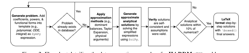Figure 2. Flowchart detailing the data generation procedure for HARDMATH problems

The exact missing link or mathematical gap that this paper attempts to bridge is the ability of LLMs to move beyond exact computation and formal reasoning to master the art of analytical approximation in applied mathematics. This involves understanding the behavior of complex functions in different regimes (e.g., small or large parameters), applying techniques like dominant balance, and making informed, justified approximations where exact solutions are unavailable. The paper explicitly states that a primary motivation is the "lack of benchmark datasets targeting the mathematical approximation methods required in many applications" (Page 1, Section 1), particularly for problems involving integrals, ordinary differential equations (ODEs), and partial differential equations (PDEs) that "do not have closed-form solutions" (Page 1, Section 1).

The painful trade-off or dilemma that has historically trapped researchers in this field, and now LLMs, is the inherent tension between mathematical precision (exact solutions) and practical utility (approximate analytical solutions). While exact solutions offer undeniable rigor, they are often impossible or intractable for real-world scientific and engineering problems. Numerical solutions provide answers but "often fail to provide intuition behind solutions behavior" (Page 1, Section 1). Applied mathematics, especially asymptotic methods, seeks approximate analytical solutions that offer crucial intuition, but these solutions require "subjective choices about the regimes of solution space to consider, the number of terms to include in approximate expressions, and the approximation methods themselves" (Page 4, Section 3.1). This blend of rigorous analysis with judicious, context-dependent judgment is exceedingly difficult to formalize and automate, presenting a significant hurdle for LLMs trained primarily on exact computations or abstract logic.

Constraints & Failure Modes

The problem of benchmarking LLMs on advanced applied mathematics, particularly those requiring approximation, is made insanely difficult by several harsh, realistic constraints and inherent failure modes:

• Mathematical Intractability and Non-Exactness: Many real-world applied mathematics problems, including integrals, ODEs, and PDEs, simply "do not have closed-form solutions" (Page 1, Section 1). This means LLMs cannot rely on finding a single, precise analytical answer. Instead, they must employ "analytical approximation techniques" (Page 1, Abstract), which are inherently more complex and less deterministic than exact calculations.
• Subjectivity and Judgment in Approximation: Unlike straightforward calculations, deriving approximate analytical solutions often involves "subjective choices about the regimes of solution space to consider, the number of terms to include in approximate expressions, and the approximation methods themselves" (Page 4, Section 3.1). These choices require deep mathematical intuition and justification, which are challenging for current LLMs to replicate.
• Lack of Suitable Training and Evaluation Data: A critical constraint is the "lack of benchmark datasets targeting the mathematical approximation methods" (Page 1, Section 1). Existing datasets are either too simple, too focused on exact solutions, or too abstract. Advanced datasets are typically "manually-sourced," making them "limited by their size and scalability" (Page 2, Section 2.1). This data sparsity for the specific problem domain makes it hard to train and evaluate LLMs effectively.
• Computational and Verification Complexity: Generating a large-scale dataset of these problems with validated solutions is a significant computational and intellectual undertaking. The authors had to develop algorithms to auto-generate problems and then validate their approximate solutions against "numerical ground truths" (Page 1, Abstract). This validation process is not trivial and involves "semi-automated human-verification" (Page 5, Section 3.2; Page 13, Figure 5), highlighting the difficulty in ensuring correctness for approximate solutions.

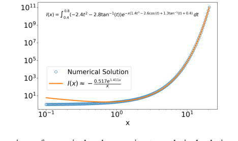Figure 5. Visual comparison of numerical and approximate analytical solutions to a sample Laplace integral problem for solution verification

• LLM Integration of Tools and Reasoning: The problems in HARDMATH are unique because their approximate solutions "cannot be formalized using tools like Lean or similar software" (Page 3, Section 2.1). This means LLMs need to "integrate tool use with sophisticated reasoning" (Page 3, Section 2.1) rather than just offloading tasks to formal solvers, which is a more advanced and less developed capability.
• Observed LLM Failure Modes: Current LLMs consistently demonstrate "significantly lower performance" on HARDMATH compared to other benchmarks (Page 1, Abstract). Detailed error analysis reveals specific failure modes:
  • Incorrect Dominant Balance Setup: LLMs often struggle to correctly identify and set up the dominant terms in an equation for different regimes (Page 9, Section 4.4; Page 29, Problem 136).
  • Missing Dominant Balance Cases: Models frequently fail to consider all relevant regimes or dominant balances, leading to incomplete solutions (Page 10, Figure 4).
  • Failure to Calculate Complex Roots/Terms: Even when the balance is correctly identified, LLMs may fail to accurately calculate the resulting approximate roots or correction terms, especially complex ones (Page 9, Section 4.4; Page 10, Figure 4).

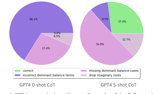Figure 4. GPT-4 error modes for problem type Roots at 0 vs. 5 shot CoT prompting

*   **Lack of Procedural Reasoning:** Some models provide only final answers without showing intermediate steps, making it difficult to trace errors and assess their reasoning path (Page 9, Section 4.4). This necessitates a "procedural grading" approach (Page 7, Section 4.1).
*   **Heuristic vs. Rigorous Approximation:** LLMs often resort to heuristic approximations without the necessary mathematical rigor, leading to less accurate or incomplete solutions compared to ground truth (Page 32, Box 5).

Why This Approach

The Inevitability of the Choice

The creation of the HARDMATH dataset, with its unique focus on algorithmically generated problems requiring approximate analytical solutions, was not merely a preference but a necessity driven by significant gaps in existing benchmarks. The authors realized that traditional "SOTA" methods for dataset creation—namely, manual curation from textbooks or competitions—were fundamentally insufficient for their specific objective.

The core issue was the underrepresentationd of advanced applied mathematics problems in Large Language Model (LLM) benchmarks. Existing datasets predominantly focused on grade-school to high-school level mathematics, or on abstract, formal university-level problems that typically have exact, "clean" analytical solutions. However, real-world scientific and engineering contexts frequently present problems involving integrals, ordinary differential equations (ODEs), and partial differential equations (PDEs) that lack closed-form solutions. These problems necessitate approximate analytical solutions derived through asymptotic and applied analysis techniques.

The "exact moment" of realization isn't pinpointed to a single event, but rather emerges from the collective observation that current LLM benchmarks fail to capture this crucial aspect of mathemtical reasoning. The paper explicitly states: "A primary motivation for developing HARDMATH is the lack of benchmark datasets targeting the mathematical approximation methods required in many applications." (Section 1). LLMs, even leading models like GPT-4, perform poorly on these types of problems (achieving only 43.8% accuracy on HARDMATH-MINI, as noted in the Abstract), indicating that existing training and evaluation paradigms are inadequate for this domain.

Therefore, the only viable solution for creating a benchmark that truly assesses LLMs' capabilities in this challenging, approximation-oriented applied mathematics domain was to develop a novel, algorithmic approach for problem generation. This was essential to overcome the limitations of manual curation, which could not provide the necessary scale, diversity, or specific problem characteristics required.

Comparative Superiority

The algorithmic generation approach employed for HARDMATH offers qualitative superiority over previous gold standards of dataset creation, extending far beyond simple performance metrics. Its structural advantages are overwhelmingly clear:

• Unprecedented Scalability: Unlike manually curated datasets, which are inherently limited in size and difficult to expand, HARDMATH's algorithmic framework allows for the automatic generation of "any number of additional problems" (Section 2.1). This is a critical advantage for continuous LLM development, fine-tuning, and benchmarking, ensuring a perpetually fresh and extensive supply of diverse problems.
• Targeted Diversity and Realism: The dataset is specifically designed to capture a "fundamentally different type of mathematical reasoning" (Section 1) compared to other benchmarks. It focuses on problems inspired by graduate-level asymptotic methods, covering algebraic equations, ODEs, and integrals that often lack exact solutions. This provides a more realistic and challenging testbed for LLMs, reflecting the complexity of problems encountered in real-world scientific research, rather than just abstract or elementary calculations.
• Evaluation of Tool Use and Sophisticated Reasoning: HARDMATH problems are unique because their approximate solutions "cannot be formalized using tools like Lean or similar software" (Section 2.1). To succeed, LLMs must "integrate tool use with sophisticated reasoning" (Section 2.1), including computational tools for numerical ground truths and analytical techniques. This structural design makes HARDMATH an invaluable benchmark for evaluating an LLM's ability to combine symbolic manipulation, numerical computation, and high-level reasoning, a capability largely unaddressed by other datasets.
• Robust and Semi-Automated Verification: The dataset generation includes "automatic numeric validity checks and an easy visual means for human-verification" (Section 5). Solutions are validated against numerical ground truths, with problems only included if their approximate solutions have less than 10% error (Section 3.2). This semi-automated process ensures a high level of confidence in solution accuracy and rigor, a significant advantage over purely manual verification which is prone to human error and impractical at scale.

Figure 2. Flowchart detailing the data generation procedure for HARDMATH problems

Alignment with Constraints

The chosen method of algorithmic problem generation for HARDMATH perfectly aligns with the inherent constraints and requirements of the problem it seeks to address, forming a strong "marriage" between the problem's harsh demands and the solution's unique properties.

1. Constraint: Addressing the Gap in Advanced Applied Mathematics: The primary constraint was the lack of benchmarks for advanced applied mathematics problems requiring approximation techniques. HARDMATH directly addresses this by algorithmically generating problems specifically focused on "asymptotic reasoning in mathematics" (Section 1), including nondimensionalization, polynomial root-finding, nonlinear ODEs, and various integrals (Section 3.1). This ensures the dataset is purpose-built for the exact type of mathematical reasoning that was missing.
2. Constraint: Need for Scalability and Broad Coverage: Existing datasets were limited in size and difficult to scale or diversify. The algorithmic generation process is the ideal solution, as it can "auto-generate a large number of problems" (Abstract) by combining randomly selected coefficients, functional forms, and initial conditions (Section 3.2). This property ensures that HARDMATH can be expanded indefinitely, providing a robust and diverse set of problems without the bottlenecks of manual curation.
3. Constraint: Problems Requiring Reasoning, Computation, and Judgment: The target problems demand a blend of "mathematical reasoning, computational tools, and subjective judgment" (Abstract). The algorithmic approach is designed to produce problems that require the "Method of Dominant Balance" and other sophisticated techniques (Section 3.1). The solutions inherently involve "subjective choices about the regimes of solution space to consider, the number of terms to include in approximate expressions, and the approximation methods themselves" (Section 3.1). This directly mirrors the complex decision-making processes involved in real-world applied mathematics, which cannot be captured by problems with straightforward, exact solutions.
4. Constraint: High-Quality and Verifiable Solutions: The need for reliable ground truths for benchmarking LLMs was paramount. The algorithmic generation is coupled with a rigorous verification process, including "automatic numeric validity checks" and "easy visual means for human-verification" (Section 5). Problems are only included if their approximate solutions are within 10% error of numerical ground truths (Section 3.2). This ensures the high quality and correctness of the solutions, which is crucial for accurate LLM evaluation.

Rejection of Alternatives

The paper clearly articulates why alternative approaches to dataset creation were deemed unsuitable for HARDMATH's specific goals, leading to the adoption of algorithmic generation.

• Manual Curation from Textbooks, Standardized Tests, or Competitions: This "typical approach" (Section 1) was explicitly rejected for several reasons:

  • Limited Scale and Scalability: Datasets derived from textbooks or similar resources are "generally quite small and difficult to broaden easily" (Section 2.1). The sheer volume and diversity of problems needed to effectively benchmark LLMs on advanced applied mathematics could not be achieved through manual collection.
  • Inadequate Problem Focus: Most existing manually curated datasets focus on "grade school- to high school-level mathematics problems" or "abstract, formal mathematics" (Section 2.1) with exact solutions. They "exclude other forms of mathematical reasoning" (Section 2.1) that involve approximation and asymptotic methods, which is the core focus of HARDMATH.
  • Copyright Issues: "textbook problems are often protected by copyright, which can complicate their public use" (Section 2.1). An algorithmically generated dataset bypasses these legal restrictions, allowing for open and widespread use.

• Formal Verification Software (e.g., Lean): The paper notes that "The problems in our dataset are unique because they involve approximate solutions that cannot be formalized using tools like Lean or similar software" (Section 2.1). This implies a fundamental incompatibility between the nature of HARDMATH's problems and the capabilities of such tools. Formal verification systems are designed for rigorous, exact proofs within formal logical frameworks. The problems in HARDMATH, however, inherently involve approximations, estimations, and "subjective judgment" (Section 3.1) in defining solution regimes or terms. This qualitative aspect of applied mathematics makes it impossible to use tools built for exact, formal reasoning. Therefore, relying on such tools for solution generation or verification would have failed to capture the essence of the problme domain.

Mathematical & Logical Mechanism

The Master Equation

The core mathematical engine powering the solutions within the HARDMATH dataset, particularly for problems involving asymptotic analysis, isn't a single universal equation but rather a methodology applied to various problem types. This methodology, primarily the Method of Dominant Balance, dictates how complex equations are simplified and solved approximately in different regimes. To illustrate this mechanism, we'll focus on a representative polynomial root-finding problem, which clearly demonstrates the application of dominant balance. The "master equation" in this context is the polynomial whose roots are sought:

$$ P(x) = \epsilon x^6 - x^5 + 1 = 0 $$

This equation, taken from the paper's examples (Section A.2.2, page 14), serves as an excellent proxy for the "transformation logic" that underpins many problems in HARDMATH. The goal is to find approximate expressions for the roots $x$ in the limits of small and large positive $\epsilon$.

Term-by-Term Autopsy

Let's dissect the chosen polynomial $P(x) = \epsilon x^6 - x^5 + 1 = 0$ to understand the role of each component in the context of asymptotic analysis. We can label the terms as $A = \epsilon x^6$, $B = -x^5$, and $C = 1$.

• $\epsilon$:

  1. Mathematical Definition: A small, positive, dimensionless parameter. It's often referred to as a "perturbation parameter" in asymptotic methods.
  2. Physical/Logical Role: This parameter controls the relative magnitude of the $\epsilon x^6$ term. Its smallness (or largeness) defines the "regimes" of the problem, where different terms in the equation become dominant. The author uses it to introduce a scaling that makes exact solutions intractable but approximate solutions possible through dominant balance.
  3. Why Addition/Multiplication: $\epsilon$ is multiplied by $x^6$ to form a single term. The terms $A, B, C$ are then added to form the polynomial, representing a sum of different physical or mathematical contributions that must collectively equal zero for a root to exist.

• $x^6$:

  1. Mathematical Definition: A monomial, $x$ raised to the power of 6.
  2. Physical/Logical Role: Represents a component of the polynomial whose magnitude scales rapidly with $x$. In conjunction with $\epsilon$, it forms a term whose dominance depends on both $x$ and $\epsilon$.
  3. Why Addition/Multiplication: It's a power of the variable $x$.

• $-x^5$:

  1. Mathematical Definition: A monomial, $x$ raised to the power of 5, with a negative coefficient.
  2. Physical/Logical Role: Another component of the polynomial, also scaling with $x$. Its negative sign indicates an opposing contribution to the sum. Its relative magnitude compared to $\epsilon x^6$ and $1$ is crucial for determining dominant balances.
  3. Why Addition/Multiplication: It's a power of $x$, added to the other terms to form the polynomial.

• $1$:

  1. Mathematical Definition: A constant term.
  2. Physical/Logical Role: Represents a baseline or a constant, non-scaling contribution to the polynomial. Its magnitude is independent of $x$ and $\epsilon$, making its relative importance vary significantly across different regimes of $x$ and $\epsilon$.
  3. Why Addition/Multiplication: It's a constant, added to the other terms.

• $= 0$:

  1. Mathematical Definition: An equality operator.
  2. Physical/Logical Role: This operator transforms the polynomial expression into an equation, defining the problem as finding the specific values of $x$ (the roots) for which the entire expression sums to zero.

The choice of addition for combining terms is fundamental to polynomial structure. The "why" behind using dominant balance (instead of, say, direct algebraic solution) is that for higher-order polynomials (quintic or higher), exact analytical root-finding formulas do not exist (Stewart, 2015). Asymptotic methods provide a powerful alternative for finding approximate solutions when exact ones are elusive, especially when a small or large parameter like $\epsilon$ is present.

Step-by-Step Flow

Let's trace the lifecycle of this abstract polynomial $P(x) = \epsilon x^6 - x^5 + 1 = 0$ as it's processed by the Method of Dominant Balance to find its roots. Imagine this as a mechanical assembly line for mathematical solutions:

1. Input & Term Identification: The polynomial $P(x)$ enters the system. The first step is to identify its constituent terms: $A = \epsilon x^6$, $B = -x^5$, and $C = 1$.
2. Regime Selection: The problem specifies regimes of interest: "small positive $\epsilon$" and "large positive $\epsilon$". Let's focus on the "small positive $\epsilon$" regime for this walkthrough.
3. Hypothesize Dominant Balances: For a three-term equation, there are three possible pairwise dominant balances, assuming the third term is negligible. The system systematically explores these:
   • Balance 1 (A and B dominate): Assume $|C| \ll |A|$ and $|C| \ll |B|$. The equation simplifies to $\epsilon x^6 - x^5 \approx 0$.
   • Balance 2 (B and C dominate): Assume $|A| \ll |B|$ and $|A| \ll |C|$. The equation simplifies to $-x^5 + 1 \approx 0$.
   • Balance 3 (A and C dominate): Assume $|B| \ll |A|$ and $|B| \ll |C|$. The equation simplifies to $\epsilon x^6 + 1 \approx 0$.
4. Solve Simplified Equations: Each hypothesized balance is now treated as a simpler equation:
   • For Balance 1: $\epsilon x^6 - x^5 = 0 \implies x^5(\epsilon x - 1) = 0$. This yields $x=0$ (a trivial root, often discarded in these contexts) and $\epsilon x - 1 = 0 \implies x = 1/\epsilon$.
   • For Balance 2: $-x^5 + 1 = 0 \implies x^5 = 1$. This yields five roots, including $x=1$ and four complex roots (e.g., $e^{i2\pi k/5}$ for $k=1,2,3,4$).
   • For Balance 3: $\epsilon x^6 + 1 = 0 \implies x^6 = -1/\epsilon$. This yields six roots, including complex roots like $x = (1/\epsilon)^{1/6} e^{i(\pi + 2\pi k)/6}$.
5. Consistency Check (The Crucial Filter): For each set of roots found, the system performs a vital check:
   • For $x = 1/\epsilon$ (from Balance 1): Substitute this $x$ back into the magnitudes of all three original terms: $|A| = |\epsilon (1/\epsilon)^6| = 1/\epsilon^5$, $|B| = |-(1/\epsilon)^5| = 1/\epsilon^5$, $|C| = |1|$. For small $\epsilon$, $1/\epsilon^5$ is very large, so $|A|$ and $|B|$ are indeed much larger than $|C|$. This balance is consistent for small $\epsilon$.
   • For $x=1$ (from Balance 2): Substitute $x=1$ into the terms: $|A| = |\epsilon (1)^6| = \epsilon$, $|B| = |-(1)^5| = 1$, $|C| = |1|$. For small $\epsilon$, $\epsilon$ is very small, so $|A| \ll |B|$ and $|A| \ll |C|$. This balance is consistent for small $\epsilon$.
   • For $x = (1/\epsilon)^{1/6} e^{i\theta}$ (from Balance 3): Substitute this $x$ into the terms: $|A| = |\epsilon (1/\epsilon)| = 1$, $|B| = |-(1/\epsilon)^{5/6}|$, $|C| = |1|$. For small $\epsilon$, $(1/\epsilon)^{5/6}$ is very large, so $|B|$ is not negligible compared to $|A|$ and $|C|$. This balance is inconsistent for small $\epsilon$.
6. Output Valid Roots: The system collects only the roots from the consistent balances for the given regime. For small $\epsilon$, the roots from Balance 1 ($x=1/\epsilon$) and Balance 2 ($x=1, e^{i2\pi k/5}$) are valid. The process is then repeated for the "large positive $\epsilon$" regime.

This systematic exploration and verification process ensures that the approximate solutions are mathematically justified within their respective asymptotic regimes, making the abstract math feel like a moving mechanical assembly line that filters and refines potential solutions.

Optimization Dynamics

The "optimization dynamics" in the context of HARDMATH's problem-solving mechanism refers to how the analytical approximation methods, particularly dominant balance and series expansions, "converge" to an accurate solution. It's not about gradient descent or a loss landscape in the machine learning sense, but rather the iterative refinement of an analytical approximation.

1. Initial Approximation (Dominant Balance): The process begins by identifying the "dominant" terms in an equation for a specific asymptotic regime (e.g., small $\epsilon$, large $x$). This is the first, often crude, approximation. It simplifies a complex equation into a solvable form. The "convergence" here is immediate: the complex problem is reduced to a simpler one.
2. Consistency Check as a Feedback Loop: After finding an approximate solution from a dominant balance, a critical step is the consistency check. This acts as a feedback mechanism. If the neglected terms are not significantly smaller than the dominant terms, the initial assumption was flawed, and the "solution" is discarded. This prevents the method from "converging" to an incorrect or invalid approximation. It's a logical check that guides the search for valid regimes.
3. Iterative Refinement (Correction Terms): For problems requiring higher accuracy, the mechanism can "learn" or "update" the solution by introducing correction terms. As seen in polynomial root correction (Section A.2.3), an initial root approximation $\bar{x}(\epsilon)$ is refined by adding a small error term $\delta$, such that $x^*(\epsilon) = \bar{x}(\epsilon) + \delta$. Plugging this ansatz back into the original equation and performing a Taylor expansion allows for solving for $\delta$, which is typically of a higher order in $\epsilon$ (or $x$). This iterative process effectively "converges" to a more precise analytical solution by accounting for previously neglected, but next-order, terms. Each iteration brings the approximate solution closer to the true solution, much like an optimization algorithm iteratively reduces loss.
4. Regime Exploration: The "state updates iteratively over time" can be seen in the exploration of different asymptotic regimes. The mechanism doesn't settle on a single solution but rather explores how the solution "state" (the form of the roots or approximations) changes as parameters like $\epsilon$ or $x$ vary significantly. This systematic exploration ensures a comprehensive understanding of the problem's behavior across its entire domain.

In essence, the "optimization" is the analytical pursuit of the most accurate and consistent approximation within defined mathematical constraints, using a series of logical steps and refinements rather than numerical gradients. The "loss landscape" is implicitly shaped by the magnitudes of the terms in the equation, where "valleys" represent consistent dominant balances and "peaks" represent inconsistent assumptions. The goal is to find the "lowest points" (most consistent approximations) in this analytical landscape.

Results, Limitations & Conclusion

Experimental Design & Baselines

To rigorously evaluate Large Language Models (LLMs) on challenging applied mathematics problems, the authors constructed HARDMATH-MINI, a carefully curated subset of 366 problems. This test set mirrors the statistical composition of the full HARDMATH dataset (1,060 problems), which is intended for model development and fine-tuning. The problems in HARDMATH-MINI are categorized into four distinct types: Nondimensionalization (symbolic and numerical), Polynomial Root-finding, Nonlinear Ordinary Differential Equations (ODEs), and Integrals (traditional and Laplace).

The experimental architecture was designed to ruthlessly prove the mathematical claims by employing a dual-pronged evaluation protocol. First, an automatic final answer assessment was used, where LLMs were prompted to enclose their final answers in \boxed{} LaTeX commands. These outputs were then compared against ground truth solutions using both SymPy-based equivalence checks and numerical evaluations, ensuring robustness against varied mathematical expression formats. Second, a novel procedural LLM-based grading approach was implemented. GPT-40 served as the "grader," prompted with ground truth answer keys and detailed rubrics adapted from course grading guidelines (Appendix A.3.2, Table 5). This procedural grading was crucial for problem types requiring complex, multi-step solutions (e.g., Laplace integral approximations) or those demanding human-like abstraction and approximation judgments, where a single exact answer is not always feasible. A manual verification of a subset of these LLM-based grades confirmed their close alignment with human judgment.

The "victims" (baseline models) included a range of both closed-source and open-source LLMs. Closed-source models comprised GPT-3.5, GPT-4, and o1-mini, while open-source models included Llama3-8b and CodeLlama-13b. These models were evaluated under zero-shot and few-shot (1-shot and 5-shot) Chain-of-Thought (CoT) prompting conditions to assess the impact of explicit reasoning steps. Additionally, a separate evaluation was conducted on 40 hand-crafted word problems, formulated in applied science contexts, using GPT-4 to gauge performance in more realistic, contextualized scenarios, deliberately omitting problem-specific hints.

What the Evidence Proves

The evidence definitively proves that current LLMs, including leading frontier models, exhibit significant limitations in solving advanced applied mathematics problems requiring analytical approximation techniques. On the HARDMATH-MINI dataset, even GPT-4, with 5-shot CoT prompting, achieved an overall accuracy of only 43.8%. The o1-mini model, despite its smaller parameter size, showed the best performance among all tested models, reaching 62.3% overall accuracy with 5-shot CoT. In stark contrast, open-source models like Llama3-8b achieved a mere 20.2% accuracy under similar conditions.

This performance is substantially lower than what these same models achieve on existing mathematics benchmarks. For instance, GPT-4's 43.8% on HARDMATH-MINI pales in comparison to its reported 72.2% accuracy on the MATH dataset (0-shot CoT) and 92.0% on GSM-8K (5-shot CoT). Similarly, o1-mini's 62.3% on HARDMATH-MINI is significantly lower than its 90.0% accuracy on MATH-500 (0-shot CoT). This stark disparity is undeniable evidence that HARDMATH poses unique and challenging tasks that go beyond the capabilities demonstrated on simpler, calculation-focused benchmarks. The core mechanism of the dataset—requiring approximate analytical solutions, dominant balance, and subjective judgment—is indeed a formidable hurdle for LLMs.

Few-shot CoT prompting consistently boosted performance across all models, with o1-mini and GPT-4 showing the most pronounced improvements. This indicates that providing explicit reasoning steps helps models, but it doesn't fully bridge the gap. A detailed error analysis (Figure 4) revealed that CoT prompting shifted error modes for problems like "Roots." Instead of making fundamental errors in setting up dominant balances, models with CoT moved to more nuanced issues, such as "missing dominant balance cases" or "failing to calculate complex roots." This suggests an improved understanding of the dominant balance technique but a continued struggle with its comprehensive and precise application.

Figure 4. GPT-4 error modes for problem type Roots at 0 vs. 5 shot CoT prompting

Problem types varied in difficulty, with ODEs proving "comparatively harder" for all models, often resulting in partial rather than full correctness. Nondimensionalization problems, conversely, were generally the "easiest." The evaluation on 40 hand-crafted word problems further underscored the challenge, with GPT-4 achieving only 28.1% accuracy, indicating that contextualizing these problems in real-world scenarios, even without additional prompt engineering, does not simplify them for LLMs. The rigorous validation of HARDMATH solutions against numerical ground truths (e.g., Figure 5) ensures that the observed LLM failures are not due to dataset inaccuracies but rather reflect genuine limitations in their mathematical reasoning abilities.

Figure 5. Visual comparison of numerical and approximate analytical solutions to a sample Laplace integral problem for solution verification

Limitations & Future Directions

While the HARDMATH dataset and its evaluation provide crucial insights, there are several limitations to acknowledge. Firstly, the current evaluation primarily uses HARDMATH-MINI as a test set, leaving the larger HARDMATH dataset (1,060 problems) largely unexplored for model fine-tuning or development. This means the full potential impact of training LLMs on such a diverse and challenging dataset has yet to be realized. Secondly, the evaluation was conducted on a specific subset of frontier models available at the time, and the landscape of LLMs is rapidly evolving. New models or improved versions could potentially alter these findings. A minor limitation noted was that o1-mini sometimes returns only final answers without intermediate steps, which makes detailed error tracing and understanding its reasoning pitfalls difficult. Lastly, the automated generation of word problem contexts, while promising, still has limitations in capturing the subtle, domain-specific priors that human experts might intuitively apply, and the current set of 40 word problems is relatively small.

Looking ahead, several exciting avenues for future development and evolution emerge from these findings:

1. Leveraging the Full HARDMATH Dataset: The most immediate next step is to fine-tune LLMs on the complete HARDMATH dataset. This could significantly improve their performance on asymptotic methods and provide a richer understanding of how LLMs learn and generalize complex mathematical reasoning.
2. Expanding Model Evaluations: As new LLMs become available, extending the evaluation to include them will provide more detailed insights into performance disparities and further advance our understanding of LLMs' capabilities in handling complex mathematical reasoning. This continuous benchmarking is vital for tracking progress in the field.
3. Refining Automated Context Generation: The automated method for generating word problems is a promising foundation. Future work should focus on refining this process to capture more subtle, domain-specific priors and expand the scale of contextualized problems. This would create a more realistic and diverse benchmark for LLMs' ability to apply math in scientific and engineering contexts.
4. Deep Dive into Error Modes: Further investigation into the fine-grained error modes, especially for models like o1-mini where intermediate steps are often omitted, is crucial. Encouraging models to consistently output their reasoning process would facilitate a more thorough analysis of their strengths and weaknesses.
5. Integrating External Tools and Symbolic Reasoning: The paper highlights that HARDMATH problems often require a combination of mathematical reasoning, computational tools, and subjective judgment. Future research could explore how LLMs can more effectively integrate external symbolic mathematics tools (like SymPy or Wolfram Alpha) to enhance their problem-solving capabilities, particularly for steps that require precise symbolic manipulation or numerical validation.
6. Developing "Human-like" Approximation Judgments: A key challenge identified is the LLMs' struggle with "human-like abstraction and approximation judgments." Future work could focus on developing models that can make more sophisticated subjective choices regarding solution regimes, the number of terms to include in approximate expressions, and the appropriate approximation methods, mirroring how human experts approach these problems. This might involve new training paradigms or architectural innovations that better capture such nuanced decision-making.
7. Exploring Multi-modal Analytical Skills: The paper mentions that graduate-level applied mathematics problems often demand "diverse, multi-modal analytical skills." This could imply integrating visual reasoning (e.g., interpreting plots like Figure 5 for solution verification) or other forms of data interpretation into LLM capabilities for solving these problems.
8. Beyond Accuracy: Interpretability and Robustness: While accuracy is important, future discussions should also consider the interpretability of LLM solutions and their robustness to variations in problem statements or numerical parameters. Can LLMs not only provide correct answers but also explain their reasoning in a way that is understandable and verifiable by human experts?

Connections to Other Fields

Mathematical Skeleton

The pure mathematical core of this work centers on the systematic application of asymptotic analysis and perturbation theory. It involves identifying dominant terms in equations or integrals under limiting conditions (e.g., small or large parameters), deriving leading-order approximate analytical solutions, and then refining these solutions through series expansions to account for smaller-order effects.

Adjacent Research Areas

Perturbation Theory in Quantum Mechanics

In quantum mechanics, perturbation theory is a foundational tool for finding approximate solutions to the Schrödinger equation when the Hamiltonian can be decomposed into an exactly solvable part and a small perturbing term. This mirrors HARDMATH's approach of finding an initial dominant balance solution and then calculating correction terms, such as the $\delta$ term for polynomial roots, using series expansions. The small parameter $\epsilon$ in HARDMATH problems is analogous to the coupling constant (e.g., the fine-structure constant $\alpha$) in quantum field theory, where physical quantities are expanded in powers of this parameter. This technique is extensively used in quantum electrodynamics and other quantum field theories (Peskin & Schroeder, 1995, An Introduction To Quantum Field Theory, Westview Press).

Singular Perturbation Theory in Fluid Dynamics

Many problems in fluid dynamics, particularly those involving high Reynolds numbers, are characterized by different behaviors in distinct spatial regions, leading to singular perturbation problems. The method of matched asymptotic expansions, a key technique within singular perturbation theory, involves constructing different asymptotic expansions valid in separate "inner" and "outer" regions, and then matching these expansions to obtain a uniformly valid approximation. This directly relates to HARDMATH's emphasis on finding approximate solutions in "small $\epsilon$" and "large $\epsilon$" regimes, or "small $x$" and "large $x$" regimes for ODEs and integrals, and the necessity to consider different dominant balances in these distinct regimes. This approach is crucial for understanding phenomena like boundary layers (Van Dyke, 1975, Perturbation Methods in Fluid Mechanics, Parabolic Press).

WKB Approximation in Wave Propagation

The Wentzel–Kramers–Brillouin (WKB) approximation is an asymptotic method used to find approximate solutions to linear ordinary differential equations with spatially varying coefficients, commonly found in wave mechanics (e.g., quantum mechanics, optics, seismology). It applies when teh wavelength of the wave changes slowly over space. The WKB method assumes a solution of an exponential form and then performs an asymptotic expansion in a small parameter (often related to the wavelength or Planck's constant). This is conceptually similar to Laplace's method for integrals, which is a form of steepest descent, where the dominant contribution comes from a specific region, and the integrand is approximated by an exponential function, leading to an asymptotic expansion. This method is a cornerstone for understanding wave phenomena in inhomogeneous media (Bender & Orszag, 2013, Advanced Mathematical Methods for Scientists and Engineers I: Asymptotic Methods and Perturbation Theory, Springer Science & Business Media).