Stability and Generalization of Stochastic Compositional Gradient Descent Algorithms

Background & Academic Lineage

The Origin & Academic Lineage

The problem addressed in this paper, Stochastic Compositional Optimization (SCO), has recently garnered significant interest within the machine learning community. This specific problem first emerged as a generalization of classic stochastic optimization. In traditional stochastic optimization, the objective function is a simple expectation. However, in SCO, the objective function takes a more complex, nested form, where an outer function operates on the expectation of an inner function. Both the inner and outer functions are themselves dependent on random variables.

This intricate structure is not merely a theoretical construct; it naturally arises in a variety of practical machine learning tasks. For instance, in reinforcement learning, the goal of obtaining a value function for a given policy can be framed as an SCO problem. Similarly, model-agnostic meta-learning (MAML), which seeks a common initialization for rapid adaptation to new tasks, is fundamentally an SCO problem. Other applications include portfolio optimization with risk aversion, addressing bias-variance issues in supervised learning, robust group distributional optimization, and maximizing performance measures like the area under precision-recall curves (AUCPRC).

Historically, a substantial body of research has focused on understanding the convergence behavior of algorithms designed to solve SCO problems. Pioneering work by Wang et al. (2017) introduced the Stochastic Compositional Gradient Descent (SCGD) algorithm and provided its non-asymptotic analysis. Subsequent studies explored accelerated versions (Wang et al., 2016), incorporated variance reduction techniques (Lian et al., 2017), developed single-timescale variants (Ghadimi et al., 2020), and introduced stochastically corrected versions like SCSC (Chen et al., 2021a). These efforts primarily aimed to demonstrate how quickly and reliably these algorithms could find an optimal solution.

The fundamental limitation, or "pain point," of these previous approaches is a significant gap in understanding their generalization properties. While we have a good grasp of how SCO algorithms converge during training, there has been very little work on understanding how these algorithms, once trained on a limited dataset, will perform on unseen or future test examples. In essence, the field lacked a comprehensive analysis of the stability and generlization capabilities of stochastic compositional optimization algorithms, despite their widespread adoption in complex machine learning tasks. This paper directly addresses this critical void by providing the first-ever known results on stability and generalization analysis for these algorithms.

Intuitive Domain Terms

To make the concepts in this paper accessible, let's translate some specialized domain terms into everyday analogies:

• Stochastic Compositional Optimization (SCO): Imagine you're trying to perfect a multi-stage manufacturing process. The final product's quality (outer function) depends on the average quality of a component (inner function), which itself is produced with some variability. SCO is like trying to optimize the settings for the entire factory line ($x$) when both the component production and final assembly steps have inherent randomness and are layered.
• Generalization: This is like a student who studies for an exam. If the student can only answer questions identical to those in their textbook (training data) but struggles with new, slightly different questions on the actual test (unseen data), they haven't "generalized" their knowledge. Good generalization means the student truly understands the underlying principles and can apply them to novel situations.
• Algorithmic Stability: Consider a chef's signature dish. If changing just one tiny ingredient in the recipe drastically alters the entire taste of the dish, it's an "unstable" recipe. An algorthm with good stability means that if you slightly change one piece of training data, the final learned model doesn't change dramatically. It's robust to minor data perturbations.
• Compositional Uniform Stability: Building on the chef analogy, imagine a complex dish where the main sauce (outer function) is made from a base stock (inner function). If you change one vegetable in the stock, how much does it affect the final dish's taste? Compositional uniform stability measures this sensitivity across both the stock's ingredients and the sauce's preparation, ensuring the entire layered process is robust to small changes. This is a more intutive form of stability for layered problems.
• Excess Risk: This term describes how much worse your algorithm performs compared to the absolute best possible performance you could ever achieve. If the "perfect" score on a game is 100, and your algorithm scores 90, its excess risk is 10. The goal is always to minimize this gap.

Notation Table

| Notation | Meaning

Problem Definition & Constraints

Core Problem Formulation & The Dilemma

The paper addresses the critical challenge of understanding generalization in Stochastic Compositional Optimization (SCO) problems. These problems are ubiquitous in modern machine learning, appearing in contexts such as reinforcement learning, AUC maximization, and meta-learning.

Input/Current State:
The starting point is a general SCO problem, where the objective function $F(x)$ has a nested compositional structure involving expectations:
$$ \min_{x \in \mathcal{X}} \left\{ F(x) = f \circ g(x) = \mathbb{E}_v \left[ f_v \left( \mathbb{E}_w [g_w(x)] \right) \right] \right\} \quad (1) $$
Here, $f: \mathbb{R}^d \to \mathbb{R}$ and $g: \mathbb{R}^p \to \mathbb{R}^d$ are differentiable functions, and $v, w$ are random variables. $\mathcal{X}$ is a convex domain in $\mathbb{R}^p$. In practical scenarios, the true population distributions of $v$ and $w$ are unknown. Instead, we are provided with finite training datasets $S_v = \{v_i : i=1, \dots, n\}$ and $S_w = \{w_j : j=1, \dots, m\}$, which are assumed to be independently and identically distributed (i.i.d.). This practical constraint transforms the population risk minimization into a nested empirical risk minimization problem:
$$ \min_{x \in \mathcal{X}} \left\{ F_S(x) := f_S(g_S(x)) = \frac{1}{n} \sum_{i=1}^n f_{v_i} \left( \frac{1}{m} \sum_{j=1}^m g_{w_j}(x) \right) \right\} \quad (2) $$
where $g_S(x) = \frac{1}{m} \sum_{j=1}^m g_{w_j}(x)$ and $f_S(y) = \frac{1}{n} \sum_{i=1}^n f_{v_i}(y)$ are the empirical counterparts of $g(x)$ and $f(y)$, respectively.

Desired Endpoint (Output/Goal State):
The ultimate goal is to rigorously analyze the excess generalization error (also known as excess risk) of a randomized algorithm $A$. This error is defined as $\mathbb{E}_{S,A}[F(A(S)) - F(x^*)]$, where $A(S)$ represents the model output by algorithm $A$ using training data $S$, and $x^*$ is the true risk minimizer, $x^* = \arg\min_{x \in \mathcal{X}} F(x)$. This excess risk is typically decomposed into two components:
$$ \mathbb{E}_{S,A}[F(A(S)) - F(x^*)] = \mathbb{E}_{S,A}[F(A(S)) - F_S(A(S))] + \mathbb{E}_{S,A}[F_S(A(S)) - F_S(x^*)] $$
The first term, $\mathbb{E}_{S,A}[F(A(S)) - F_S(A(S))]$, is the generalization gap or estimation error, quantifying how well the model performs on unseen data compared to its performance on the training data. The second term, $\mathbb{E}_{S,A}[F_S(A(S)) - F_S(x^*)]$, is the optimization error, measuring how close the algorithm's output is to the empirical risk minimizer.

Exact Missing Link or Mathematical Gap:
While there has been substantial research on the convergence behavior (optimization error) of SCO algorithms, there is a significant mathematical gap in understanding their generalization properties. Specifically, how well these algorithms, trained on finite data, perform on future, unseen test examples remains largely unexplored. The paper aims to bridge this gap by introducing a novel stability concept, "compositional uniform stability," tailored for the nested structure of SCO problems, and establishing its quantitative relationship with generalization error within the framework of statistical learning theory.

The Dilemma:
The central dilemma that has "trapped" previous researchers is the painful trade-off between optimizing for empirical risk (convergence) and ensuring strong generalization performance. In many machine learning settings, improving one aspect often comes at the expense of the other. For SCO problems, this dilemma is exacerbated by the complex compositional structure and the presence of two sets of random variables ($v$ and $w$). Existing generalization analyses for standard (non-compositional) stochastic optimization algorithms, such as SGD, do not directly extend to the SCO setting, leaving a crucial theoretical void. The challenge lies in developing algorithms that not only converge efficiently but also provide robust performance on unseen data, a property not guaranteed by convergence alone.

Constraints & Failure Modes

The problem of analyzing stability and generalization for SCO algorithms is inherently difficult due to several harsh, realistic constraints:

1. Complex Compositional Structure: The nested expectation in $F(x) = \mathbb{E}_v [f_v (\mathbb{E}_w [g_w(x)])]$ is the primary source of difficulty. Unlike standard stochastic optimization, the objective function involves an "inner" expectation $\mathbb{E}_w [g_w(x)]$ and an "outer" expectation $\mathbb{E}_v [f_v(\cdot)]$. This structure makes it non-trivial to define and analyze algorithmic stability, as perturbations in training data can affect both inner and outer functions.
2. Defining Compositional Stability: A major constraint was the absence of a suitable stability definition for compositional settings. The paper introduces "compositional uniform stability" (Definition 2.1), but relating this new concept to the generalization error requires intricate mathematical derivations, particularly concerning the decoupling of inner and outer random variables.
3. Inability to Interchange Expectation and Norm: As noted in the paper (page 5), a significant technical challenge arises when dealing with terms like $\mathbb{E}_{S,A} [\|g(A(S)) - \frac{1}{m} \sum_{j=1}^m g_{w_j}(A(S))\|]$. The expectation and norm operators cannot be freely interchanged, which complicates direct analysis. This necessitates advanced techniques like sample-splitting arguments to overcome this mathematical barrier.
4. Increased Variance Terms: The stability bounds derived for SCO algorithms (SCGD and SCSC) contain additional variance terms compared to non-compositional SGD. These include the empirical variance associated with the inner function $g_w$ and terms related to the convergence of the moving average sequence $Y_{t+1}$ to track $g_S(x_t)$. These extra terms make the analysis more involved and require careful balancing with optimization errors.
5. High Computational Cost (Iterations): Achieving the desired excess risk rates, such as $O(1/\sqrt{n} + 1/\sqrt{m})$, for SCO algorithms demands a substantially larger number of iterations ($T$) than for their non-compositional counterparts. For instance, in the convex setting, SCGD requires $T = \max(n^{3.5}, m^{3.5})$ iterations, and SCSC needs $T = \max(n^{2.5}, m^{2.5})$. In the strongly convex case, these requirements escalate to $T = \max(n^{10/3}, m^{10/3})$ for SCGD and $T = \max(n^{7/3}, m^{7/3})$ for SCSC. This translates to a significant computational burden, potentially limiting real-world applicability in settings with strict latency requirements.
6. Assumptions on Function Properties: The current analysis relies on strong assumptions, including Lipschitz continuity of $f_v$ and $g_w$ (Assumption 2.2), Lipschitz continuity of their gradients (Assumption 3.1), and convexity or strong convexity of the objective function $F_S$. Relaxing these assumptions to non-convex, non-smooth, or more complex function classes (e.g., neural networks with ReLU activations) presents further formidable challenges, which are explicitly left for future research.
7. Data Perturbation Complexity: The definition of compositional uniform stability requires considering "neighboring" datasets where a single data point is changed. Due to the dual nature of random variables ($v$ and $w$), this perturbation can occur in either $S_v$ or $S_w$, adding a layer of complexity to tracking the algorithm's sensitivity to data changes.
8. Dimension-Independent Bounds: A specific constraint for this work was to derive dimension-independent generalization bounds. Previous work (e.g., Hu et al., 2020) often yielded bounds that were heavily dependent on the dimension of the optimization domain $\mathcal{X}$, making them less practical for high-dimensional problems. Achieving dimension independence is a non-trivial task that adds to the problem's difficulty.

Why This Approach

The Inevitability of the Choice

The adoption of compositional uniform stability within the framework of statistical learning theory was not merely a choice but an inevitability for addressing the generalization properties of stochastic compositional optimization (SCO) algorithms. The authors explicitly state that while significant research has focused on the convergence behavior of SCO algorithms, there has been "little work on understanding their generlization" (Abstract, page 1). Traditional "SOTA" methods for analyzing generalization, such as those applied to standard Stochastic Gradient Descent (SGD) or other algorithms in the non-compositional Empirical Risk Minimization (ERM) setting, were inherently insufficient.

The exact moment this insufficiency became apparent stems from the unique structure of SCO problems, where the objective function involves a nested composition of functions, each associated with an expectation (Introduction, page 1). This two-level randomness and compositional structure fundamentally differ from the single-level expectation and non-compositional nature of classical stochastic optimization problems. Existing stability concepts, like uniform argument stability or on-average model stability, were developed for these simpler, non-compositional settings (Related Work, page 2). They simply do not account for the intricate interplay between the inner and outer functions, nor the distinct random variables ($v$ and $w$) associated with each level of composition. Therefore, a novel stability concept, specifically "compositional uniform stability," was the only viable solution to quantitatively relate the learning algorithm's behavior on training data to its performance on unseen test examples in this complex setting.

Comparative Superiority

The proposed analysis approach demonstrates qualitative superiority beyond simple performance metrics by offering a framework uniquely suited to the structural complexities of SCO problems. Its primary structural advantage lies in the introduction of "compositional uniform stability," a concept specifically "tailored to handle the composition structure in SCO problems" (Our Contributions, page 2). Unlike previous gold standards in generalization analysis for non-compositional settings, this new definition (Definition 2.1, page 4) explicitly considers how changes in either the outer function's data ($S_v$) or the inner function's data ($S_w$) affect the algorithm's output. This granular understanding of stability, accounting for both levels of randomness, is a profound qualitative leap.

Furthermore, the method yields "dimension-independent excess risk bounds" for the analyzed algorithms (SCGD and SCSC) (Abstract, page 1, and Remark 3.8, page 7). This is a critical advantage over prior work, such as that by Hu et al. (2020), whose bounds were "highly dependent on the dimension of the domain $X \subseteq R^P$" (Remark 3.8, page 7). Achieving dimension independence implies that the analysis is more robust and broadly applicable, especially in high-dimensional machine learning tasks, without suffering from a quadratic or higher dependency on the problem's dimensionality.

Quantitatively, the analysis also reveals that the SCSC algorithm, a stochastically corrected version of SCGD, requires significantly fewer iterations to achieve the same excess risk rate. For instance, in the convex setting, SCSC needs $T = \max(n^{2.5}, m^{2.5})$ iterations, whereas SCGD requires $T = \max(n^{3.5}, m^{3.5})$ (Table 1, page 7). This translates to a substantial reduction in computational complexity, making SCSC a more efficient choice for practical applications, a direct outcome of this detailed stability and generalization analysis.

Alignment with Constraints

The chosen method, centered on compositional uniform stability, perfectly aligns with the inherent constraints and unique properties of stochastic compositional optimization (SCO) problems. The "marriage" between the problem's harsh requirements and the solution's unqiue properties is evident in several aspects:

1. Nested Composition: SCO problems are defined by their nested function structure, $f \circ g$. The proposed "compositional uniform stability" directly addresses this by introducing a stability concept that explicitly accounts for this composition (Our Contributions, page 2).
2. Dual Expectations: The objective function involves expectations over two sets of random variables, $v$ and $w$. Definition 2.1 of compositional uniform stability reflects this by considering neighboring datasets where a single data point is changed in either $S_v$ or $S_w$ (page 4). This dual consideration is crucial for accurately capturing the problem's stochastic nature at both levels.
3. Generalization Goal: The overarching problem constraint is to understand generalization for SCO algorithms. Theorem 2.3 (page 4) directly establishes a quantitative relationship between the defined compositional uniform stability and the generalization error, making the analysis framework purpose-built for this goal.
4. Mathematical Properties: The analysis relies on standard assumptions like Lipschitz continuity for both inner and outer functions (Assumption 2.2, page 4), which are common and necessary properties in SCO optimization literature. The framework is designed to leverage these properties, for example, by using the Lipschitz property of $f_v$ to handle vector-valued generalization terms (page 5).
5. Computational Challenges: The compositional structure introduces specific technical challenges, such as the inability to directly interchange expectation and norm for vector-valued inner functions. The authors address this by employing a sample-splitting argument (Bousquet et al., 2020; Lei, 2022), demonstrating how the analysis adapts to these computational intricacies (Our Contributions, page 2, and page 5).

Rejection of Alternatives

The paper implicitly and explicitly rejects alternative generalization analysis approaches by highlighting their limitations when applied to the stochastic compositional optimization (SCO) setting. The core argument for rejecting alternatives is that existing methods primarily focus on the non-compositional setting, which fails to capture the unique nested structure and dual stochasticity of SCO problems.

Specifically:
* Standard SGD Generalization Analysis: The authors repeatedly emphasize that "existing work of stability analysis... focused on SGD algorithms in the non-compositional ERM setting" (Section 2.2, page 4). While these methods are effective for simpler problems, directly applying them to SCO would be insufficient. The paper demonstrates this by showing that if the inner function $g_w(x) = x$, the SCO problem reduces to the non-compositional setting, and their compositional stability results match those of SGD (Remark 2.4, page 4, and Remark 3.4, page 6). This implies that a non-compositional analysis would miss the "two extra terms" that arise from the compositional structure, which are crucial for understanding generalization in the full SCO context (Remark 3.4, page 6).
* Algorithm-Independent Bounds (Hu et al., 2020): The work by Hu et al. (2020) studied generalization for the exact minimizer of the ERM counterpart for SCO using uniform convergence. However, their bounds were "algorithm-independent" and "highly dependent on the dimension of the domain $X \subseteq R^P$" (Remark 3.8, page 7). The current paper's approach, by contrast, provides algorithm-dependent bounds for specific SCO algorithms (SCGD and SCSC) and, more importantly, achieves dimension-independent excess risk bounds. This qualitative advantage demonstrates why Hu et al.'s approach, while valuable, would have been less informative for the specific goal of analyzing algorithmic generalization in a dimension-agnostic manner.

The paper does not discuss the failure of deep learning architectures like GANs or Diffusion models, as its scope is on the theoretical analysis of optimization algorithms for SCO, not on specific model types. The rejection of alternatives is thus rooted in the inadequacy of existing theoretical frameworks to handle the compositional and dual-stochastic nature of the problem at hand.

Mathematical & Logical Mechanism

The Master Equation

At the heart of this paper's approach to solving Stochastic Compositional Optimization (SCO) problems lies an iterative update mechanism for the model parameters. While the ultimate goal is to minimize the population risk $F(x)$ (Equation 1 in the paper), the algorithms operate on the empirical risk $F_S(x)$ (Equation 2). The core mathematical engine is the stochastic gradient descent update rule for the model parameter $x$, combined with a moving average sequence $Y_t$ that approximates the inner expectation.

The master equation for updating the model parameter $x$ at each iteration $t$ is given by:
$$ x_{t+1} = \Pi_{\mathcal{X}}(x_t - \eta_t \nabla g_{w_{j_t}}(x_t) \nabla f_{v_{i_t}}(Y_{t+1})) $$
This equation is common to both Stochastic Compositional Gradient Descent (SCGD) and Stochastically Corrected Stochastic Compositional Gradient Descent (SCSC) algorithms. The key difference between these two algorithms lies in how the intermediate moving average $Y_{t+1}$ is computed.

For SCGD, the update for $Y_{t+1}$ is:
$$ Y_{t+1} = (1 - \beta_t)Y_t + \beta_t g_{w_{j_t}}(x_t) $$
For SCSC, which incorporates a variance reduction technique, the update for $Y_{t+1}$ is:
$$ Y_{t+1} = (1 - \beta_t)(Y_t + g_{w_{j_t}}(x_t) - g_{w_{j_t}}(x_{t-1})) + \beta_t g_{w_{j_t}}(x_t) $$

Term-by-Term Autopsy

Let's dissect the master equation and its auxiliary updates to understand the role of each component.

In the main update equation $x_{t+1} = \Pi_{\mathcal{X}}(x_t - \eta_t \nabla g_{w_{j_t}}(x_t) \nabla f_{v_{i_t}}(Y_{t+1}))$:

• $x_{t+1}$: This is the model parameter vector at iteration $t+1$. Its mathematical definition is simply the output of the current update step. Its physical/logical role is the new candidate solution for the optimization problem, aiming to minimize the objective function.
• $\Pi_{\mathcal{X}}(\cdot)$: This is the projection operator onto the convex domain $\mathcal{X}$. Mathematically, it maps any point outside $\mathcal{X}$ to the closest point within $\mathcal{X}$. Its physical/logical role is to ensure that the updated model parameters $x_{t+1}$ always remain within the predefined feasible set $\mathcal{X}$, which is a common constraint in many optimization problems.
• $x_t$: This is the model parameter vector at iteration $t$. It represents the current state of our solution.
• $\eta_t$: This is the learning rate or step size at iteration $t$. Mathematically, it's a positive scalar that scales the gradient. Its physical/logical role is to control the magnitude of the step taken in the direction of the negative gradient. A carefully chosen $\eta_t$ (often decreasing over time) is crucial for convergence. The paper often considers $\eta_t = \eta$ for simplicity in its analysis.
• $\nabla$: This is the gradient operator. Mathematically, it computes the vector of partial derivatives of a function. Its physical/logical role is to indicate the direction of the steepest ascent of a function. In minimization, we move in the opposite direction.
• $g_{w_{j_t}}(x_t)$: This represents the inner function $g$ evaluated at $x_t$ with a randomly sampled $w_{j_t}$. Mathematically, it's a vector-valued function $g: \mathbb{R}^p \to \mathbb{R}^d$. Its physical/logical role is to provide a stochastic, single-sample estimate of the inner expectation $\mathbb{E}_w[g_w(x_t)]$.
• $\nabla g_{w_{j_t}}(x_t)$: This is the gradient (Jacobian) of the inner function $g$ with respect to $x_t$, evaluated at $x_t$ with $w_{j_t}$. Mathematically, it's a matrix (Jacobian) that transforms vectors from the output space of $g$ to its input space. Its physical/logical role is to apply the chain rule, effectively translating the gradient of the outer function (which operates on $g(x)$'s output) back into the parameter space of $x$.
• $\nabla f_{v_{i_t}}(Y_{t+1})$: This is the gradient of the outer function $f$ with respect to its input, evaluated at $Y_{t+1}$ with a randomly sampled $v_{i_t}$. Mathematically, it's a vector-valued function $f: \mathbb{R}^d \to \mathbb{R}$. Its physical/logical role is to provide a stochastic, single-sample estimate of the gradient of the outer function, evaluated at the current approximation of the inner expectation.
• Multiplication ($\nabla g_{w_{j_t}}(x_t) \nabla f_{v_{i_t}}(Y_{t+1})$): This is a matrix-vector product (or Jacobian-vector product). Its physical/logical role is to compute the stochastic gradient of the compositional function $f(g(x))$ with respect to $x$, following the chain rule. This is the estimated direction of steepest ascent for the overall objective.
• Subtraction ($x_t - \dots$): This is vector subtraction. Its physical/logical role is to move the parameter $x_t$ in the direction opposite to the estimated gradient, which is the fundamental operation for minimizing a function using gradient descent.

Now, for the auxiliary update equations for $Y_{t+1}$:

For SCGD: $Y_{t+1} = (1 - \beta_t)Y_t + \beta_t g_{w_{j_t}}(x_t)$
* $Y_{t+1}$: This is the moving average sequence at iteration $t+1$. Mathematically, it's a weighted average of past values. Its physical/logical role is to serve as a smoothed, low-variance approximation of the inner expectation $\mathbb{E}_w[g_w(x_t)]$. This smoothing helps stabilize the overall gradient estimate.
* $\beta_t$: This is the step size for the moving average update at iteration $t$. Mathematically, it's a positive scalar. Its physical/logical role is to control the weight given to the new stochastic sample $g_{w_{j_t}}(x_t)$ versus the previous moving average $Y_t$. The paper often considers $\beta_t = \beta$.
* $Y_t$: This is the moving average sequence at iteration $t$. It represents the previous approximation of the inner expectation.
* $g_{w_{j_t}}(x_t)$: (Already explained above).
* Addition and coefficients $(1-\beta_t)$, $\beta_t$: These form a convex combination, ensuring that $Y_{t+1}$ is a stable and weighted average of the past estimate and the new sample. This is a standard technique for reducing the variance of stochastic estimates.

For SCSC: $Y_{t+1} = (1 - \beta_t)(Y_t + g_{w_{j_t}}(x_t) - g_{w_{j_t}}(x_{t-1})) + \beta_t g_{w_{j_t}}(x_t)$
* This equation introduces a stochastically corrected term for variance reduction.
* $(1 - \beta_t)(Y_t + g_{w_{j_t}}(x_t) - g_{w_{j_t}}(x_{t-1}))$: This part represents a corrected version of the previous moving average. The term $g_{w_{j_t}}(x_t) - g_{w_{j_t}}(x_{t-1})$ is a difference that accounts for the change in the inner function's output due to the parameter update from $x_{t-1}$ to $x_t$. Its physical/logical role is to act as a control variate, reducing the variance of the estimate for $\mathbb{E}_w[g_w(x_t)]$ by leveraging information from the previous step. This makes the estimate $Y_{t+1}$ more accurate and stable.
* $\beta_t g_{w_{j_t}}(x_t)$: This is the weighted current stochastic sample, similar to SCGD, incorporating the latest information.
* Addition: Combines the corrected old estimate with the new sample.

The choice of addition for combining terms in the moving average and subtraction for gradient descent is standard. The multiplication of gradients is a direct application of the chain rule for derivatives of composite functions. The use of summations in the empirical risk (Equation 2) reflects the averaging over discrete training samples, as opposed to integrals for continuous population distributions.

Step-by-Step Flow

Let's trace the journey of an abstract data point through one iteration of these algorithms, imagining it as a mechanical assembly line.

1. Initialization: We start an iteration $t$ with the current model parameter $x_t$ (and $x_{t-1}$ for SCSC) and the previous moving average $Y_t$.
2. Stochastic Sampling: The first station on our assembly line is the "Data Sampler." Here, a single data point $v_{i_t}$ is randomly drawn from the outer dataset $S_v$, and another data point $w_{j_t}$ is randomly drawn from the inner dataset $S_w$. These are the raw materials for our stochastic estimates.
3. Inner Function Evaluation: The raw data $w_{j_t}$ and the current parameter $x_t$ are fed into the "Inner Function Processor," which computes $g_{w_{j_t}}(x_t)$. For SCSC, the previous parameter $x_{t-1}$ is also used to compute $g_{w_{j_t}}(x_{t-1})$.
4. Moving Average Update (The Inner Estimator):
   • SCGD Path: The computed $g_{w_{j_t}}(x_t)$ and the previous moving average $Y_t$ enter the "SCGD Smoother." They are blended using the step size $\beta_t$: $Y_{t+1} = (1 - \beta_t)Y_t + \beta_t g_{w_{j_t}}(x_t)$. This new $Y_{t+1}$ is a smoothed, low-variance estimate of the inner expectation.
   • SCSC Path: For SCSC, the "SCSC Corrector" takes $Y_t$, $g_{w_{j_t}}(x_t)$, and $g_{w_{j_t}}(x_{t-1})$. It first calculates a correction term $g_{w_{j_t}}(x_t) - g_{w_{j_t}}(x_{t-1})$ and then combines it: $Y_{t+1} = (1 - \beta_t)(Y_t + g_{w_{j_t}}(x_t) - g_{w_{j_t}}(x_{t-1})) + \beta_t g_{w_{j_t}}(x_t)$. This is a more sophisticated smoothing, designed to reduce variance more effectively.
5. Outer Gradient Computation: The newly computed $Y_{t+1}$ (from either path) and the sampled $v_{i_t}$ are sent to the "Outer Gradient Engine." This engine calculates the gradient of the outer function, $\nabla f_{v_{i_t}}(Y_{t+1})$.
6. Inner Gradient Computation: Simultaneously, the current parameter $x_t$ and the sampled $w_{j_t}$ go to the "Inner Gradient Engine," which computes $\nabla g_{w_{j_t}}(x_t)$.
7. Chain Rule Multiplier: The outputs from the Outer and Inner Gradient Engines, $\nabla f_{v_{i_t}}(Y_{t+1})$ and $\nabla g_{w_{j_t}}(x_t)$, converge at the "Chain Rule Multiplier." Here, they are multiplied to produce the full stochastic compositional gradient: $\nabla g_{w_{j_t}}(x_t) \nabla f_{v_{i_t}}(Y_{t+1})$. This is our estimated direction for parameter adjustment.
8. Parameter Adjuster: The current parameter $x_t$ and the stochastic gradient are fed into the "Parameter Adjuster." It takes a step in the negative direction of the gradient, scaled by the learning rate $\eta_t$: $x_t - \eta_t (\text{stochastic gradient})$.
9. Projection Unit: Finally, the adjusted parameter enters the "Projection Unit." If it falls outside the feasible domain $\mathcal{X}$, this unit projects it back onto the boundary, ensuring the parameter remains valid. The output of this unit is $x_{t+1}$.
10. Loop: The updated $x_{t+1}$ (and $Y_{t+1}$) are then fed back to the start of the assembly line for the next iteration, repeating the process until a stopping criterion is met.

This mechanical flow iteratively refines the model parameters, guided by stochastic estimates of the compositional gradient.

Optimization Dynamics

The optimization dynamics of SCGD and SCSC algorithms are centered around iteratively navigating a complex loss landscape defined by the stochastic compositional objective function. The core idea is to minimize this objective by following estimated gradients, with specific mechanisms to handle the nested expectation structure and reduce variance.

1. Loss Landscape: The objective function $F_S(x)$ (or $F(x)$ in the ideal population setting) represents a multi-dimensional loss landscape. In the convex and strongly convex settings analyzed in the paper, this landscape is generally well-behaved, resembling a bowl. The goal is to find the lowest point (minimum) in this bowl. Strong convexity implies a steeper, more pronounced bowl, which typically allows for faster convergence to the minimum.

2. Stochastic Gradients: Instead of computing the exact gradient of $F_S(x)$ (which would be computationally expensive, requiring averaging over all $n$ outer samples and $m$ inner samples), these algorithms rely on stochastic gradients. At each iteration, only a single $v_{i_t}$ and $w_{j_t}$ are sampled to estimate the gradient. This introduces noise (variance) into the gradient direction but drastically reduces the computational cost per step, making it feasible for large datasets. The algorithms then take small steps in the opposite direction of this noisy gradient.

3. Two-Timescale Updates: A critical aspect of these algorithms is their two-timescale update rule. This is a common strategy for nested optimization problems.

   • Faster Timescale (Inner Variable $Y_t$): The moving average $Y_t$ is designed to track the inner expectation $\mathbb{E}_w[g_w(x_t)]$ relatively quickly. The step size $\beta_t$ for $Y_t$ is typically chosen to be larger or to decay slower than the step size for $x_t$, allowing $Y_t$ to rapidly adapt to changes in $x_t$ and provide a good approximation of the inner expectation. This ensures that the outer gradient $\nabla f_{v_{i_t}}(Y_{t+1})$ is evaluated at a reasonably accurate point.
   • Slower Timescale (Outer Variable $x_t$): The model parameter $x_t$ is updated with a smaller or more slowly decaying learning rate $\eta_t$. This slower update allows the inner estimate $Y_t$ to "catch up" and stabilize before $x_t$ takes a substantial step. This separation of timescales is vital for the overall stability and convergence of the algorithm, preventing oscillations that could arise if both variables updated too quickly based on noisy estimates.

4. Variance Reduction (SCSC): The SCSC algorithm introduces a clever variance reduction technique within its $Y_t$ update. The term $g_{w_{j_t}}(x_t) - g_{w_{j_t}}(x_{t-1})$ acts as a control variate. By subtracting the inner function's value at the previous parameter $x_{t-1}$ and adding it at the current $x_t$, SCSC effectively reduces the variance of the estimate for $\mathbb{E}_w[g_w(x_t)]$. This leads to more accurate gradient estimates for the outer function, which in turn results in a smoother, more direct path towards the minimum in the loss landscape. The paper's results show that SCSC requires fewer iterations (e.g., $T = \max(n^{2.5}, m^{2.5})$ for convex cases) to achieve the same excess risk rate compared to SCGD ($T = \max(n^{3.5}, m^{3.5})$), directly demonstrating the benefit of this variance reduction.

5. Convergence and Stability: The iterative updates, driven by these stochastic gradients and two-timescale dynamics, aim to converge to a minimizer of the empirical risk. The paper's primary focus is on the stability of these algorithms, which quantifies how much the algorithm's output changes when a single training data point is perturbed. High stability is directly linked to good generalization performance – meaning the model trained on the finite dataset $S$ will perform well on unseen test data. The careful selection of step sizes $\eta_t$ and $\beta_t$ (often as decaying functions of the total iterations $T$, like $\eta = T^{-a}$ and $\beta = T^{-b}$) is crucial for balancing the optimization error (how close the algorithm gets to the empirical minimum) and the generalization error (the gap between empirical and true risk). The analysis shows that by balancing these factors, the algorithms achieve dimension-independent excess risk bounds, a significant theoretical result. The iterative process continues for a predetermined number of iterations $T$, or until a convergence criterion is met, with the final output being either the last iterate $x_T$ or an average of intermediate iterates.

Results, Limitations & Conclusion

Experimental Design & Baselines

The analysis presented in this paper is primarily theoretical, focusing on establishing mathematical bounds for stability and generalization rather than conducting empirical experiments with specific datasets or hardware. Therefore, the "experimental design" here refers to the rigorous theoretical framwork and the comparative methodology employed to validate the authors' claims.

The core of their theoretical "experiment" was to introduce and analyze a novel concept called "compositional uniform stability" (Definition 2.1), specifically tailored to address the nested function structure inherent in Stochastic Compositional Optimization (SCO) problems. This new stability definition serves as the foundation for deriving generalization bounds for SCO algorithms.

The "victims" (baseline models) against which the proposed algorithms, Stochastic Compositional Gradient Descent (SCGD) and Stochastically Corrected Stochastic Compositional Gradient Descent (SCSC), were theoretically compared include:

• Standard Stochastic Gradient Descent (SGD) in the non-compositional setting: This is the most prominent baseline. The authors repeatedly compare their derived stability bounds for SCGD and SCSC to the well-known $O(1/\sqrt{n})$ uniform stability results for SGD in convex and smooth settings (e.g., Hardt et al., 2016). This comparison ruthlessly highlights the additional complexities introduced by the compositional structure.
• Existing SCO convergence analyses: Prior work on SCO algorithms predominantly focused on convergence rates (e.g., Wang et al., 2017; Chen et al., 2021a). This paper extends the analysis to generalization, thus implicitly "defeating" the limitation of previous studies by providing a more complete theoretical understanding.
• Exact Empirical Risk Minimizer (ERM) for SCO: Hu et al. (2020) studied generalization for the exact ERM minimizer of SCO. However, their bounds were algorithm-independent and often dimension-dependent. The present work aims to provide algorithm-specific and dimension-independent bounds for SCGD and SCSC, thereby offering a more practical and robust analysis for these specific algorithms.

The authors architected their theoretical validation by:
1. Defining compositional uniform stability.
2. Establishing a quantitative relationship between this new stability concept and the generalization error (Theorem 2.3).
3. Deriving explicit compositional uniform stability bounds for SCGD and SCSC under both convex (Theorem 3.3, Corollary 3.5) and strongly convex (Theorem 3.11, Corollary 3.13) settings.
4. Combining these stability bounds with optimization error bounds (Theorem 3.6, Theorem 3.14) to finally obtain dimension-independent excess risk bounds for SCGD and SCSC (Theorem 3.7, Theorem 3.15). This multi-step mathematical derivation serves as the definitive, undeniable evidence that their core mechanism—compositional uniform stability—actually works in reality to characterize generalization for SCO problems.

What the Evidence Proves

The evidence, in the form of rigorous mathematical theorems and corollaries, definitively proves several key aspects of the authors' claims:

• Validation of Compositional Uniform Stability: Theorem 2.3 is the cornerstone, establishing a clear quantitative link between the newly introduced compositional uniform stability and the generalization error (gap) for any randomized SCO algorithm. This theorem validates that their stability definition is indeed a suitable metric for analyzing generalization in compositional settings. The presence of a variance term, $\text{Var}_w(g_w(A(S)))$, in the generalization bound (Theorem 2.3) highlights the unique challenge of SCO problems, which is directly addressed by their stability concept.
• Definitive Evidence of Core Mechanism: The paper successfully derives explicit compositional uniform stability bounds for SCGD and SCSC. For instance, in the convex setting, Corollary 3.5 provides bounds for $\epsilon_v + \epsilon_w$ for both algorithms, demonstrating how the compositional structure introduces additional terms related to the inner function's variance and the moving average sequence's convergence (Remark 3.4). This is undeniable evidence that their framework captures the nuances of SCO generalization.
• Superiority of SCSC over SCGD in Iteration Complexity:
  • Convex Setting (Theorem 3.7): To acheive an excess risk rate of $O(1/\sqrt{n} + 1/\sqrt{m})$, SCGD requires approximately $T = \max(n^{3.5}, m^{3.5})$ iterations. In stark contrast, SCSC only needs $T = \max(n^{2.5}, m^{2.5})$ iterations. This is a definitive victory for SCSC, showing it can reach the same generalization performance with significantly fewer computational steps.
  • Strongly Convex Setting (Theorem 3.15): Similarly, for the strongly convex case, to achieve an excess risk rate of $O(1/n + 1/\sqrt{m})$, SCGD demands about $T = \max(n^{10/3}, m^{10/3})$ iterations, while SCSC requires a lower $T = \max(n^{7/3}, m^{7/3})$ iterations. Again, SCSC demonstrates superior iteration efficiency.
• Dimension-Independent Excess Risk Bounds: A significant achievement is the derivation of excess risk bounds that are independent of the dimension of the optimization domain $X \subseteq \mathbb{R}^p$ (Remark 3.8). This is a crucial improvement over prior work (e.g., Hu et al., 2020) where bounds were often dimension-dependent, making the current results more broadly applicable and robust.

Limitations & Future Directions

This paper makes a substantial theoretical contribution, but like all scientific endeavors, it operates within certain boundaries and opens avenues for future exploration.

Current Limitations:

• Convex and Smooth Assumptions: The most significant limitation is that the entire analysis, including stability and generalization bounds, is restricted to convex and smooth objective functions (Section 4, Remark 3.16). Many real-world machine learning problems, especially those involving deep neural networks, are inherently non-convex and/or non-smooth. This restricts the direct applicability of the current theoretical results to such complex scenarios.
• Suboptimal Time Complexity: While the paper establishes generalization rates, it notes that the iteration complexities required for SCGD and SCSC (e.g., $T = \max(n^{3.5}, m^{3.5})$ in the convex case) are still far from the optimal linear time complexity $T = O(\max(n, m))$ that would be desirable for practical efficiency (Section 4).
• Independent Random Variables: The primary analysis assumes that the random variables $v$ and $w$ (associated with the outer and inner functions, respectively) are independent (Section 2.1). Although Appendix E briefly discusses the "coupled" case where $v$ and $w$ exhibit interdependence, detailed proofs and a full analysis for this more complex and often realistic scenario are deferred to future work.

Future Directions & Discussion Topics:

1. Extending to Non-convex and Non-smooth Settings: How can the compositional uniform stability framwork be adapted or extended to analyze SCO problems with non-convex and/or non-smooth objective functions? This would be a major leap, potentially requiring new definitions of stability (e.g., based on weak convexity or specific neural network architectures like those with ReLU activations, as mentioned in Remark 3.16). What novel mathematical techniques would be necessary to handle the increased complexity of non-convex landscapes in a compositional context?
2. Achieving Optimal Time Complexity: Given the current iteration complexities, what algorithmic innovations or theoretical breakthroughs could enable SCGD and SCSC (or their variants) to acheive optimal excess risk rates with linear time complexity, i.e., $T = O(\max(n, m))$? This might involve more advanced variance reduction techniques, adaptive step-size strategies, or entirely new optimization paradigms specifically designed for compositional problems.
3. Multi-level Compositional Optimization: The paper hints at multi-level composition problems as a future direction (Section 4). How would the concepts of stability and generalization extend to problems with three or more nested functions, each potentially associated with its own expectation? What new challenges arise in defining stability, decomposing generalization error, and deriving bounds for such hierarchical structures?
4. Rigorous Analysis of Coupled Compositional SCO: The brief discussion in Appendix E on coupled compositional SCO (where $v$ and $w$ are dependent) highlights a cruical area for future work. What specific mathematical tools are needed to rigorously analyze stability and generalization when these random variables are interdependent? Could techniques from causal inference, graphical models, or advanced stochastic calculus be integrated to model and bound the effects of such dependencies?
5. Empirical Validation and Practical Impact: While this paper is theoretical, its findings have implications for practical applications like reinforcement learning, meta-learning, and AUC maximization. What empirical studies would be most effective in validating the theoretical iteration complexity differences between SCGD and SCSC? How can these theoretical insights guide practitioners in choosing or designing more efficient and generalizable SCO algorithms for real-world tasks, especially as problem sizes ($n, m$) grow?
6. Beyond Uniform Stability: The paper focuses on compositional uniform stability. Are there other notions of algorithmic stability (e.g., data-dependent stability, on-average model stability) that could provide tighter or more nuanced generalization bounds for SCO problems under different data distributions or model complexities? Exploring these alternative stability concepts might offer deeper insights into the generalization behavior of compositional algorithms.

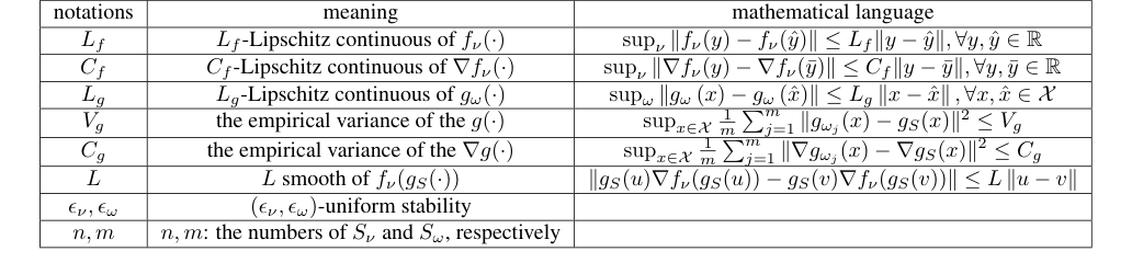Table 2. Notations notations meaning mathematical language Lf Lf-Lipschitz continuous of fν(·) supν ∥fν(y) −fν(ˆy)∥≤Lf∥y −ˆy∥, ∀y, ˆy ∈R Cf Cf-Lipschitz continuous of ∇fν(·) supν ∥∇fν(y) −∇fν(¯y)∥≤Cf∥y −¯y∥, ∀y, ¯y ∈R Lg Lg-Lipschitz continuous of gω(·) supω ∥gω (x) −gω (ˆx)∥≤Lg ∥x −ˆx∥, ∀x, ˆx ∈X Vg the empirical variance of the g(·) supx∈X 1 m Pm j=1 ∥gωj(x) −gS(x)∥2 ≤Vg Cg the empirical variance of the ∇g(·) supx∈X 1 m Pm j=1 ∥∇gωj(x) −∇gS(x)∥2 ≤Cg L L smooth of fν(gS(·)) ∥gS(u)∇fν(gS(u)) −gS(v)∇fν(gS(v))∥≤L ∥u −v∥ ϵν, ϵω (ϵν, ϵω)-uniform stability n, m n, m: the numbers of Sν and Sω, respectively 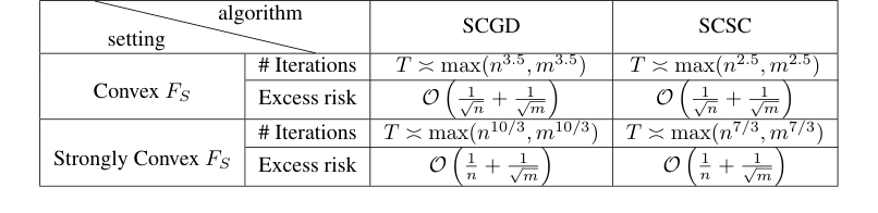Table 1. Number of Iterations T that Achieves Excess Risk for SCGD And SCSC Algorithm

Connections to Other Fields

Mathematical Skeleton

The pure mathematical core of this work lies in extending the concept of uniform stability from classical empirical risk minimization to stochastic compositional optimization problems. It rigorously defines a new notion, "compositional uniform stability," and establishes a quantitative relationship between this stability measure and the generalization error, specifically for algorithms that handle nested expectations.

Adjacent Research Areas

Statistical Learning Theory & Algorithmic Stability

This paper directly builds upon and significantly extends the foundational work in statistical learning theory, particularly in the realm of algorithmic stability. The introduction of "compositional uniform stability" (Definition 2.1) is a direct, technically rigorous adaptation of the well-established uniform stability concept (e.g., as defined in Bousquet & Elisseeff, 2002) to address the unique nested structure of stochastic compositional optimization (SCO) problems. The core proof technique, which involves bounding the change in an algorithm's output when a single data point in the training set is perturbed, is a canonical method in stability analysis. Theorem 2.3, which quantifies the connection between compositional uniform stability and generalization error, is a direct generalization of similar results in non-compositional settings, providing a deeper understanding of how learning algorthms generalize in more complex scenarios.
Representative Paper: Hardt, M., Recht, B., & Singer, Y. (2016). Train faster, generalize better: Stability of stochastic gradient descent. International Conference on Machine Learning.

Stochastic Optimization Algorithms

The work provides a theoretical underpinning for a class of stochastic optimization algorithms, specifically Stochastic Compositional Gradient Descent (SCGD) and its stochastically corrected variant (SCSC). The analysis of their stability and generlization properties directly contributes to the broader field of stochastic optimization. The algorithms themselves employ techniques common in stochastic approximation, such as two-time scale updates and moving averages, to efficiently estimate gradients in the presence of nested expectations. The paper's methodology of decomposing the excess risk into optimization and generalization errors, and then bounding each term, is a standard and rigorous approach in the theoretical analysis of stochastic optimization methods. This allows for a comprehensive understanding of the trade-offs involved in designing and analyzing such algorithms.
Representative Paper: Wang, M., Fang, E. X., & Liu, H. (2017). Stochastic compositional gradient descent: algorithms for minimizing compositions of expected-value functions. Mathematical Programming.

Reinforcement Learning & Meta-Learning

The problem formulation of stochastic compositional optimization (SCO) directly models several important tasks in reinforcement learning (RL) and meta-learning. For instance, in RL, the objective function often involves nested expectations, such as when estimating value functions where the outer expectation is over states and the inner is over future rewards or actions. Similarly, meta-learning, particularly model-agnostic meta-learning (MAML), can be cast as an SCO problem where the goal is to find an initialization that performs well across a distribution of tasks, each involving an expectation over local data. The stability and generalization guarantees derived in this paper for SCO algorithms thus provide crucial theoretical insights into why and how these learning paradigms perform well on unseen data or tasks, extending beyond just convergence analysis to address the critical aspect of generalization.
Representative Paper (RL): Sutton, R. S., & Barto, A. G. (2018). Reinforcement learning: An introduction. MIT press.
Representative Paper (Meta-Learning): Finn, C., Abbeel, P., & Levine, S. (2017). Model-agnostic meta-learning for fast adaptation of deep networks. International conference on machine learning.