
Oscillatory behavior for higher-order nonlinear differential equations in the canonical case
In this paper, we study the oscillation of a class of higher-order neutral nonlinear differential equations.
Background & Academic Lineage
The Origin & Academic Lineage
The problem addressed in this paper, concerning the oscillatory behavior of higher-order neutral nonlinear differential equations (NDEs) in the canonical case, stems from a fundamental challenge in mathematics and its applications: the inability to find explicit, closed-form solutions for a vast number of differential equations (DEs). Historically, the focus in studying DEs was often on obtaining exact solutions. However, as models became more complex, particularly in physics, engineering, and biology (e.g., celestial mechanics, neural dynamics, population dynamics), it became clear that many DEs simply don't have such neat solutions.
This "pain point" led to the emergence of qualitative theory for DEs, a field dedicated to understanding the behavior of solutions without necessarily knowing their exact form. This theoretical framework traces its origins to the pioneering works of Henri Poincare and Alexandre Lyapunov in the late 19th and early 20th centuries. Their contributions laid the groundwork for analyzing properties like stability, periodicity, and, crucially, oscillation.
Within this qualitative realm, oscillation theory specifically investigates whether solutions to DEs fluctuate recurrently around a central value (oscillatory) or eventually settle down to a constant or monotonic trend (non-oscillatory). The particular class of equations, Neutral Differential Equations (NDEs), arose to model systems exhibiting "memory effects." Unlike Ordinary Differential Equations (ODEs), where the rate of change depends only on the present state, NDEs incorporate past states (delayed values) into their derivative. This makes them particularly relevant for phenomena where historical data significantly impacts current and future behavior, such as in certain biological or control systems.
The fundamental limitation or "pain point" of previous approaches that compelled the authors to write this paper is the insufficiency of existing oscillation criteria for the specific class of higher-order neutral nonlinear differential equations they investigate. While there has been significant progress in oscillation theory for various types of DEs, including those with delay arguments and NDEs of both odd and even orders, the authors explicitly state that their work aims to "improve upon related results in the literature." They seek to establish "novel oscillation criteria involving a single condition" that are more general and effective. For instance, in their examples, they demonstrate that previously established theorems (e.g., Theorem 2 from [28] and Theorem 1 from [25]) fail to determine the oscillatory nature of certain equations, whereas their new criteria successfully do. This highlights that prior methods were not robust enough to cover the full spectrum of conditions or equation structures, leaving a gap that this paper endeavors to fill with more comprehensive and simplified criteria.
Intuitive Domain Terms
Here are a few specialized terms from the paper, translated into everyday analogies:
- Differential Equation (DE): Imagine you're trying to describe how a car moves. A Differential Equation is like a detailed instruction manual that tells you how the car's speed and position change at any given moment, based on its current speed, how hard you're pressing the gas, and other factors. It's a mathematical recipe for change.
- Oscillation Theory: Think about a child on a swing. Oscillation Theory is like the study of whether that swing will keep going back and forth forever (oscillatory) or if it will eventually slow down and stop at the bottom (non-oscillatory). It's about predicting if something will repeatedly fluctuate or settle down.
- Neutral Differential Equation (NDE): This is a special kind of "change recipe" where the car's acceleration (how its speed changes) doesn't just depend on its current speed, but also on its speed from, say, five seconds ago. It's like a system with a memory, where past events directly influence the immediate future.
- Riccati Substitution: This is a clever mathematical trick, much like putting on special glasses to see a hidden pattern. When you have a very complicated equation, a Riccati substitution can transform it into a simpler, first-order inequality. This new, simpler form is often much easier to analyze, helping researchers figure out if the original system will oscillate. It's a tool to simplify and reveal.
Notation Table
| Notation | Type | Description |
|---|---|---|
Problem Definition & Constraints
Core Problem Formulation & The Dilemma
The central problem addressed by this paper is to determine the oscillatory behavior of solutions to a specific class of higher-order neutral nonlinear differential equations (NDEs).
The Input/Current State is a given NDE of the form:
$$ \left(h(s) \left(u^\beta (s) + p(s) u(\eta(s))\right)^{(n-1)}\right)' + g(s, u(\mu(s))) = 0, \quad s \geq s_0 $$
This equation comes with several crucial assumptions (A1)-(A5) on the functions and parameters involved:
* (A1) $n$ is an even natural number, and $\beta, \gamma$ are quotients of odd positive integers with $0 < \beta < 1$.
* (A2) $\mu(s), \eta(s) \in C([s_0, \infty), \mathbb{R})$, $\mu(s) \leq s$, $\mu'(s) > 0$, $\eta(s) \leq s$, $\eta'(s) > 0$, and $\lim_{s \to \infty} \mu(s) = \lim_{s \to \infty} \eta(s) = \infty$.
* (A3) $p \in C([s_0, \infty))$, $0 \leq p(s) < 1$.
* (A4) $h \in C^1([s_0, \infty), \mathbb{R}^+)$, $h'(s) \geq 0$, and $\Omega(s, s_0) := \int_{s_0}^s \frac{1}{h^{1/\beta}(\theta)} d\theta \to \infty$ as $s \to \infty$.
* (A5) $g \in C([s_0, \infty) \times \mathbb{R}, \mathbb{R})$ and there exists a function $q \in C([s_0, \infty), [0, \infty))$, $q$ does not vanish identically on any half-line of the form $[s^*, \infty)$ for $s^* \geq s_0$, such that $g(s, u) \geq q(s) u^\gamma$, where $\gamma$ is a quotient of odd positive integers.
A "solution" $u(s)$ is defined as a function $u \in C^{(n-1)}([s_u, \infty), \mathbb{R})$ that satisfies the equation on $[s_u, \infty)$ for some $s_u \geq s_0$. The paper specifically considers "proper solutions" where $\sup\{|u(s)| : s > s^*\} > 0$ for every $s^* \geq s_u$. A solution is deemed "oscillatory" if it has infinitely many zeros on $[s_u, \infty)$, meaning for any $s_1 \geq s_u$, there exists $s_2 \geq s_1$ such that $u(s_2) = 0$. If all solutions of the equation are oscillatory, the equation itself is called oscillatory.
The Desired Endpoint (Output/Goal State) is to establish a set of sufficient conditions (oscillation critera) that, when satisfied by the given NDE, guarantee that all its solutions are oscillatory. This is achieved by proving that under these conditions, no non-oscillatory (i.e., eventually positive or eventually negative) solutions can exist.
The Missing Link or Mathematical Gap this paper attempts to bridge is the absence of simple, yet powerful, analytical criteria to definitively classify the oscillatory behavior of this complex class of NDEs. Given that these equations often lack explicit closed-form solutions, direct analysis is impossible. The paper seeks to provide a rigorous mathematical framework, primarily through Riccati substitution and integral inequalities, to transform the problem of finding solutions into verifying a set of integral conditions that are easier to check.
The Painful Trade-off or Dilemma that has historically trapped researchers in this field is the difficulty in deriving oscillation criteria that are both generall enough to apply to a broad class of NDEs and sufficiently sharp (not overly restrictive) to be useful in practice. Previous criteria often involved multiple conditions or were too weak to cover certain cases, as demonstrated by the examples in this paper where earlier theorems fail. The dilemma is balancing the complexity of the underlying differential equation with the desire for simple, verifiable conditions that provide a strong guarantee of oscillation. Finding a "single condition" criterion, as the authors aim for, is a significant challenge, as improving one aspect (simplicity) often compromises another (generality or tightness).
Constraints & Failure Modes
The problem of analyzing higher-order neutral nonlinear differential equations presents several harsh, realistic walls that make it insanely difficult to solve:
-
Inherent Mathematical Complexity:
- Nonlinearity: The presence of terms like $u^\beta(s)$ and $g(s, u(\mu(s)))$ makes the equation nonlinear, which generally precludes the existence of explicit, closed-form solutions. This forces reliance on qualitative analysys, which is inherently more abstract and challenging.
- Higher-Order Derivatives: Dealing with the $(n-1)$-th derivative within the neutral term and the overall $n$-th order nature of the equation significantly complicates the analysis, requiring careful handling of multiple derivatives and integral transformations.
- Neutral Type with Delay Arguments: The "neutral" aspect means the derivative depends on delayed values of the unknown function and its derivative. This introduces "memory effects" into the system, making its behavior more intricate and less predictable than ordinary differential equations. The delay functions $\mu(s)$ and $\eta(s)$ add further complexity, as their properties (e.g., $\mu(s) \leq s$, $\eta(s) \leq s$, tending to infinity) must be carefully integrated into the analysis.
- Integral Conditions: The criteria often involve integral conditions (e.g., $\Omega(s, s_0) \to \infty$, or the conditions in Theorems 3, 4, and 5). Evaluating these integrals analytically can be difficult, and their convergence properties are critical.
-
Analytical Constraints:
- Lack of Explicit Solutions: As mentioned, the primary constraint is that these equations typically do not admit explicit solutions. This means researchers cannot simply solve the equation and observe its behavior. Instead, they must develop indirect analytical methods, such as Riccati transformations and integral inequalities, to infer qualitative properties like oscillation. This requires a deep understanding of functional analysis and differential equations theory.
- Riccati Transformation Challenges: The Riccati transformation is a powerful tool, but its application often leads to complex integral inequalities that are hard to manipulate and evaluate. Deriving a contradiction from the assumption of a non-oscillatory solution requires precise bounds and careful algebraic steps, as seen in the lengthy proofs of the theorems.
-
Comparison with Existing Literature:
- A significant "wall" is the need to improve upon existing oscillation criteria. This means the new conditions must be either more general, easier to verify, or provide stronger guarantees than previously published results. The paper explicitly shows that prior theorems (e.g., Theorem 1 from [25] and Theorem 2 from [28]) fail to establish oscillation for certain examples where the authors' new criteria succeed. This highlights the limitations of previous approaches and the difficulty in formulating universally applicable criteria.
Failure Modes for the proposed criteria would include:
* False Positives: If the derived conditions are met, but a non-oscillatory solution still exists. The paper aims to provide sufficient conditions, meaning if they are met, oscillation is guaranteed. The proofs are designed to rule out non-oscillatory solutions.
* Inapplicability: If a given NDE does not satisfy the specific assumptions (A1)-(A5) or the integral conditions derived in the theorems, then the criteria cannot be applied, and the oscillatory behavior of that particular equation remains undetermined by this method.
* Computational Intractability of Conditions: While the criteria are analytical, verifying the integral conditions (e.g., in Theorem 3, 4, or 5) for specific functions $h, p, q, \mu, \eta$ might still require complex calculations or numerical integration, especially for a zero-base reader. The goal is to make them "easier to check" than solving the DE directly, but "easy" is relative.
* Weakness for other cases: Although the authors improve upon some existing results, it's possible that for other classes of NDEs or different parameter ranges, these new criteria might still be too restrictive or not as sharp as other specialized methods.
Why This Approach
The Inevitability of the Choice
The selection of the Riccati transformation technique, coupled with a strategic application of inequalities, was not merely one option among many, but rather an indispensable approach for tackling the specific challenges posed by higher-order neutral nonlinear differential equations in the canonical case. The core problem, as highlighted in the introduction, is that many differential equations (DEs) of this complexity do not yield explicit closed-form solutions. In such scenarios, direct analytical solutions are unattainable, rendering traditional methods of finding exact solutions ineffective.
The authors implicitly recognized the insufficiency of relying solely on direct integration or standard solution techniques for these intricate equations. Instead, the focus shifted to qualitative theory, which investigates the behavior of solutions without necessarily finding them explicitly. The Riccati substitution provides a powerful framework within qualitative analysys to transform a higher-order differential equation into a first-order Riccati-type inequality. This transformation is crucial because it allows for the derivation of sufficient conditions for oscillation, a key qualitative property, by analyzing the behavior of the transformed inequality. This method becomes the only viable path when explicit solutions are elusive, as it offers a robust analytical tool to infer solution characteristics.
Comparative Superiority
The chosen methodology demonstrates clear qualitative superiority over previous gold standards, as evidenced by its ability to establish oscillation criteria where earlier results fall short. While this domain does not involve concepts like high-dimensional noise or memory complexity reduction from $O(N^2)$ to $O(N)$, the structural advantage lies in the generality and effectiveness of the derived oscillation critera.
The paper explicitly benchmarks its approach against existing results, notably those presented in [25] and [28]. For instance, in Example 2, the authors demonstrate that for a specific higher-order neutral differential equation (43), the conditions of Theorem 2 (representing a previous method) are not satisfied, thus failing to determine its oscillatory behavior. In stark contrast, the proposed Theorem 5 successfully establishes that equation (43) is oscillatory. Similarly, Example 3 illustrates that Theorem 1 (another prior result) fails to satisfy its conditions for equation (44), whereas the new Corollary 1 confirms its oscillatory nature.
This qualitative superiority stems from the novel formulation of the Riccati substitution and the accompanying inequalities, which are more finely tuned to the specific structure of the higher-order neutral nonlinear differential equations under study. The new criteria, often presented as a single, comprehensive condition, are more encompassing and less restrictive than previous multi-condition approaches, allowing for a broader range of equations to be analyzed effectively. This structural advantage makes the current method overwhelmingly superior for the class of problems considered.
Alignment with Constraints
The chosen method perfectly aligns with the inherent constraints and characteristics of the problem defined for equation (1) and its accompanying assumptions (A1-A5). The "marriage" between the problem's requirements and the solution's unqiue properties is evident in several ways:
- Higher-Order Nature (A1): The Riccati transformation is adept at reducing the complexity of higher-order derivatives, allowing the problem to be analyzed through a first-order inequality, which is more manageable.
- Neutral Delay Terms (A2, A3): The method is specifically designed to handle neutral differential equations, where the derivative depends on delayed values of the dependent variable and its derivative. The inequalities derived are tailored to accommodate the properties of the delay functions $\mu(s)$ and $\eta(s)$, and the coefficient $p(s)$.
- Nonlinearity (A5): The use of inequalities is particularly effective for nonlinear terms like $g(s,u) \geq q(s)u^\gamma$, as it allows for bounding and comparison arguments that are crucial for establishing oscillation criteria without requiring explicit solutions for the nonlinearities.
- Canonical Case (A4): The specific form of $h(s)$ and its integral properties in the canonical case are directly incorporated into the Riccati substitution and subsequent derivations, ensuring the criteria are applicable to the problem's defined scope.
- Qualitative Analysis: Given the constraint that explicit solutions are often unavailable, the method's ability to provide sufficient conditions for oscillation, a qualitative property, directly addresses the need to understand solution behavior without direct computation.
The intricate interplay between the assumptions (A1-A5) and the steps of the Riccati transformation, combined with the careful application of lemmas and inequalities, ensures that the derived oscillation criteria are precisely suited to the specific class of equations under investigation.
Rejection of Alternatives
The paper implicitly, yet effectively, rejects alternative approaches by demonstrating their limitations through concrete examples. In this field, "alternatives" refer to previously established oscillation criteria for similar classes of differential equations. The authors do not discuss methods like GANs or Diffusion models, as they are entirely outside the scope of qualitative theory for differential equations.
The primary "rejection" mechanism is found in Examples 2 and 3:
* Rejection of Theorem 2 (from [28]): For equation (43), the authors show that the condition (11) of Theorem 2, which involves the integral of $\Psi(\theta)$, is not satisfied. This means Theorem 2 cannot conclude oscillation for this specific equation.
* Rejection of Theorem 1 (from [25]): Similarly, for equation (44), the authors demonstrate that condition (6) of Theorem 1, involving a sum of integrals, is not satisfied. Consequently, Theorem 1 fails to establish oscillation for this equation.
In both instances, the proposed criteria (Theorem 5 and Corollary 1, respectively) successfully prove the oscillatory behavior of the equations. This direct comparison serves as a compelling argument for the superiority and broader applicability of the new approach. The reasoning behind rejecting these alternatives is not that they are fundamentally flawed, but rather that their conditions are too restrictive or not sufficiently general to cover the specific cases handled by the current study, thus limiting their utility for the class of equations considered here. The new method provides improved and more robust conditions that overcome these limitations.
Mathematical & Logical Mechanism
The Master Equation
The core mechanism for establishing oscillation criteria in this paper revolves around a Riccati-type transformation applied to the original higher-order neutral nonlinear differential equation (NDE). While the NDE itself (equation (1) in the paper) is the subject of study, the powering equation for the analysis is the differential inequality derived for the transformed function $\Phi(s)$. This inequality, specifically equation (29) from the paper, encapsulates the dynamic behavior that, when integrated, leads to the oscillation conditions.
The master equation is:
$$ \Phi'(s) \leq -q(s) \left[ 1 - p(\mu(s)) - \frac{(1-\beta)}{c_1} \right] \frac{\Upsilon(\mu(s))}{\beta^\gamma} - \frac{\delta N (\mu(s))^{n-2} \alpha \mu'(s)}{h^{1/\delta}(s)} \Phi^{(\delta+1)/\delta}(s) $$
Term-by-Term Autopsy
Let's dissect each component of this crucial inequality:
-
$\Phi'(s)$: This term represents the first derivative of the Riccati-type function $\Phi(s)$ with respect to the independent variable $s$.
- Mathematical Definition: $\Phi'(s) = \frac{d\Phi}{ds}$. The function $\Phi(s)$ itself is defined in equation (20) as $\Phi(s) = \frac{h(s) (y^{(n-1)}(s))^\delta}{\gamma^\delta (\alpha\mu(s))}$.
- Physical/Logical Role: It dictates the instantaneous rate of change of the transformed solution behavior. The goal of the analysis is to show that this rate of change is sufficiently negative over time, leading to a contradiction if an eventually positive solution is assumed.
- Why $\leq$: The inequality sign ($\leq$) is fundamental. The authors are deriving sufficient conditions for oscillation. This means they are finding an upper bound for $\Phi'(s)$. If this upper bound is shown to lead to a contradiction, then the actual $\Phi'(s)$ (which is even smaller or equal) must also lead to a contradiction.
-
$-q(s) \left[ 1 - p(\mu(s)) - \frac{(1-\beta)}{c_1} \right] \frac{\Upsilon(\mu(s))}{\beta^\gamma}$: This entire first term on the right-hand side represents a "driving force" that pushes $\Phi(s)$ downwards.
- Mathematical Definition:
- $q(s)$: A continuous, non-negative function from assumption (A5), where $g(s, u) \geq q(s)u^\gamma$.
- $p(\mu(s))$: A continuous function from assumption (A3), $0 \leq p(s) < 1$, evaluated at the delayed argument $\mu(s)$.
- $\beta$: A constant, quotient of odd positive integers, $0 < \beta < 1$ (A1).
- $c_1$: A positive real constant (page 6, after (17)), arising from the lower bound of $y(s)$.
- $\Upsilon(\mu(s))$: A piecewise function defined on page 4, providing a lower bound for terms involving powers of $y(s)$, evaluated at $\mu(s)$.
- $\gamma$: A constant, quotient of odd positive integers (A5).
- Physical/Logical Role: This term aggregates the influence of the non-linear term $g(s, u(\mu(s)))$ from the original NDE (via $q(s)$ and $\gamma$) and the neutral delay term $p(s)u(\eta(s))$ (via $p(\mu(s))$ and $\beta$). The bracketed term $\left[ 1 - p(\mu(s)) - \frac{(1-\beta)}{c_1} \right]$ is expected to be positive under the conditions for oscillation, making the entire term negative due to the leading minus sign. It acts as a continuous "drain" on $\Phi(s)$.
- Why Subtraction: The subtraction indicates that these factors contribute to a decrease in $\Phi(s)$. The authors aim to show that these negative contributions are strong enough to force $\Phi(s)$ to eventually become negative, contradicting the assumption of a positive solution.
- Mathematical Definition:
-
$- \frac{\delta N (\mu(s))^{n-2} \alpha \mu'(s)}{h^{1/\delta}(s)} \Phi^{(\delta+1)/\delta}(s)$: This is the second, non-linear term on the right-hand side, which also contributes to the decrease of $\Phi(s)$.
- Mathematical Definition:
- $\delta$: A constant, quotient of odd positive integers, $0 < \delta < 1$ (A1).
- $N$: A positive constant from Lemma 3 (page 5).
- $\mu(s)$: A delay function (A2), $\mu(s) \leq s$, $\mu'(s) > 0$.
- $n$: An even natural number (A1), the order of the NDE.
- $\alpha$: A constant from Lemma 3, $a \in (0,1)$.
- $h^{1/\delta}(s)$: A function from assumption (A4), $h \in C^1([s_0, \infty), \mathbb{R}^+)$, $h'(s) \geq 0$.
- $\Phi^{(\delta+1)/\delta}(s)$: The Riccati function $\Phi(s)$ raised to the power $(\delta+1)/\delta$.
- Physical/Logical Role: This term arises from applying Lemma 4 (an inequality for $Bw - Aw^{(\delta+1)/\delta}$) and other algebraic manipulations. It represents a "self-damping" or "feedback" mechanism, where the rate of decrease of $\Phi(s)$ is proportional to a non-linear power of $\Phi(s)$ itself. Since $\Phi(s)$ is assumed positive, this term is also negative, reinforcing the downward trend. The constants $N$ and $\alpha$ are introduced by Lemma 3, which provides bounds on derivatives, while $h(s)$ is a coefficient from the original NDE. The exponent $(\delta+1)/\delta$ makes this a non-linear Riccati-type term.
- Why Subtraction: Similar to the first term, this term is subtracted because it contributes to the decrease of $\Phi(s)$. The non-linear dependence on $\Phi(s)$ is characteristic of Riccati equations and is crucial for the analytical techniques used.
- Mathematical Definition:
Step-by-Step Flow
The mathematical engine of this paper operates like a carefully constructed assembly line, transforming the problem of analyzing an NDE into a solvable inequality. Here's how an abstract data point (representing a solution $u(s)$) flows through this mechanism:
- Input: An Assumed Solution: We begin by assuming that the original higher-order NDE (1) has an eventually positive solution $u(s)$. This is the "data point" we want to process. The entire mechanism aims to show this assumption leads to a contradiction.
- First Transformation: Neutralization: The input $u(s)$ is immediately transformed into a new function $y(s) = u^\beta(s) + p(s) u(\eta(s))$. This step effectively "neutralizes" the delay term $p(s)u(\eta(s))$ by incorporating it into the definition of $y(s)$, simplifying the structure of the equation.
- Derivative Analysis (Lemma 1): The properties of $y(s)$ are then analyzed using Lemma 1. This "inspection station" determines that $y'(s) > 0$, $y^{(n-1)}(s) > 0$, and crucially, that the derivative of the highest-order term, $(h(s)(y^{(n-1)}(s))^\delta)'$, is non-positive. This establishes a monotonic behavior for key components.
- Riccati Substitution: The Core Transformation: Next, the system applies the central Riccati-type substitution. A new function $\Phi(s) = \frac{h(s) (y^{(n-1)}(s))^\delta}{\gamma^\delta (\alpha\mu(s))}$ is defined. This is like "re-encoding" the solution's properties into a form amenable to differential inequality analysis. The denominator is a specific choice to facilitate later algebraic steps.
- Differentiation of $\Phi(s)$: The $\Phi(s)$ function then passes through a "differentiation unit" where its derivative $\Phi'(s)$ is computed. This involves the chain rule and quotient rule, bringing in terms like $h'(s)$, $y^{(n)}(s)$, and $\mu'(s)$.
- Substitution and Inequality Application: This is where the "heavy lifting" occurs.
- The original NDE (1) is used to substitute for the term $(h(s)(y^{(n-1)}(s))^\delta)'$ within the $\Phi'(s)$ expression.
- Various lemmas (Lemma 2, Lemma 3, Lemma 4) are applied to bound other terms. For example, Lemma 3 provides a lower bound for derivatives like $y'(as)$, and Lemma 4 offers a powerful inequality to handle non-linear terms involving $\Phi(s)$ itself.
- Algebraic manipulations and previously derived inequalities (like (16), (18), (23), (24)) are used to simplify and bound the expression for $\Phi'(s)$.
- Output: The Riccati Inequality (29): The result of these transformations and applications is the master differential inequality (29). This inequality provides an upper bound for $\Phi'(s)$ in terms of $q(s)$, $p(\mu(s))$, $\Upsilon(\mu(s))$, $h(s)$, $\mu(s)$, and $\Phi(s)$ itself. It's a critical intermediate product, showing that $\Phi'(s)$ is bounded by negative terms.
- Integration to Infinity: The final stage involves integrating the inequality (29) from some point $s$ to infinity. This "accumulation" step sums up the negative contributions to $\Phi'(s)$ over an infinite horizon.
- Contradiction and Oscillation: If the integral of the right-hand side of (29) diverges to $-\infty$ (as specified in conditions like Theorem 3 (14) or Theorem 5 (36)), while $\Phi(s)$ is assumed to be eventually positive and bounded, a contradiction arises. This contradiction means the initial assumption of an eventually positive solution was false. Therefore, all solutions to the original NDE (1) must be oscillatory. This completes the lifecycle of the abstract data point, proving the oscillation criteria.
Optimization Dynamics
This paper's mechanism does not involve "optimization" in the typical sense of minimizing a loss function or iteratively updating parameters. Instead, it employs a proof-by-contradiction strategy rooted in qualitative analysis of differential equations. The "dynamics" here refer to the behavior of the transformed Riccati function $\Phi(s)$ and how its properties are leveraged to establish oscillation criteria.
- Loss Landscape and Convergence: There is no explicit "loss landscape" or iterative "convergence" to a minimum. The objective is not to find an optimal solution but to prove a qualitative property (oscillation) for all solutions. The "convergence" is conceptual: the argument converges to a contradiction.
- Gradient Behavior: The "gradient" in this context is $\Phi'(s)$, the rate of change of the Riccati function. The entire analytical framework is designed to show that $\Phi'(s)$ is consistently and sufficiently negative.
- The inequality (29) demonstrates that $\Phi'(s)$ is bounded from above by a sum of two negative terms.
- The first term, $-q(s) \left[ 1 - p(\mu(s)) - \frac{(1-\beta)}{c_1} \right] \frac{\Upsilon(\mu(s))}{\beta^\gamma}$, acts as a "driving force" that continuously decreases $\Phi(s)$. Its magnitude depends on the strength of the non-linear term $q(s)$ and the influence of the neutral delay $p(\mu(s))$. If $q(s)$ is large enough or $p(\mu(s))$ is small enough, this term will be strongly negative.
- The second term, $-\frac{\delta N (\mu(s))^{n-2} \alpha \mu'(s)}{h^{1/\delta}(s)} \Phi^{(\delta+1)/\delta}(s)$, provides a non-linear "self-regulating" or "damping" effect. Since $\Phi(s)$ is assumed to be positive, this term is also negative, further accelerating the decrease of $\Phi(s)$. The higher the value of $\Phi(s)$, the more negative this term becomes, creating a strong negative feedback loop.
- Iterative State Updates: There are no iterative updates in the algorithm. The proof is a direct, deductive argument. The "state" of the system, represented by $\Phi(s)$, is analyzed for its long-term behavior. If the conditions derived from integrating (29) (e.g., Theorem 3 or Theorem 5) are met, it implies that the accumulated negative contributions to $\Phi'(s)$ are so large that $\Phi(s)$ must eventually become negative. This directly contradicts the initial assumption that $\Phi(s)$ (and thus $u(s)$) remains positive. The "learning" here is not an adaptive process but a logical deduction: by understanding the combined effect of the NDE's terms on the transformed function $\Phi(s)$, the authors "learn" the conditions under which oscillation is guaranteed. This method provides a robust analytical tool for predicting oscillatory behavior without needing to solve the equation explicitly.
Results, Limitations & Conclusion
Experimental Design & Baselines
The experimental validation in this paper is purely analytical, focusing on demonstrating the applicability and improved efficacy of the proposed oscillation criteria through carefully constructed examples. There isn't a traditional experimental setup involving data collection or simulations; instead, the "experiments" are the application of the derived theorems to specific differential equations (DEs) with chosen parameters.
The authors architected their validation by presenting three illustrative examples of higher-order neutral nonlinear differential equations (NDEs). For each example, they define the specific form of the DE and assign concrete values or functional forms to its parameters, such as $h(s)$, $p(s)$, $\eta(s)$, $q(s)$, $\mu(s)$, and $\gamma(s)$. They then select an appropriate auxiliary function $\psi(\theta)$ (as required by their theorems) and rigorously evaluate whether their established oscillation conditions are met.
The "victims" (baseline models) they aimed to defeat were existing oscillation criteria from previous literature. Specifically:
* Example 2 (Equation (43)) was used to demonstrate an improvement over Theorem 2 by Althubiti et al. [28].
* Example 3 (Equation (44)) was used to show an improvement over Theorem 1 by Althubiti et al. [25].
For these comparisons, the authors meticulously showed that their novel criteria (Theorem 5 for Example 2, and Corollary 1 for Example 3) successfully predicted oscillation by satisfying the required integral conditions. Simultaneously, they demonstrated that the corresponding baseline theorems (Theorem 2 and Theorem 1, respectively) failed to satisfy their own conditions for the exact same DEs and parameters, thus being unable to conclude oscillation. This direct contrast provides the definitive, undeniable evidence that their core mechanism—the Riccati transformation technique combined with specific inequalities to derive new sufficient conditions—actually worked in reality and offered a broader scope of applicability. Visual evidence was also provided through Figure 1 and Figure 2, which graphically illustrate the behavior of the integrals involved in the oscillation conditions, confirming that the authors' conditions diverged to infinity as required, while the baseline conditions did not.
What the Evidence Proves
The evidence presented through the analytical examples definitively proves several key points regarding the authors' novel oscillation criteria for higher-order neutral nonlinear differential equations:
- Applicability and Effectiveness: The examples demonstrate that the derived theorems (Theorem 3, Theorem 4, Theorem 5, and Corollary 1) are indeed applicable to a specific class of higher-order NDEs. For the chosen examples, the criteria successfully establish the oscillatory behavior of solutions.
- Improved Scope: The most compelling evidence lies in the direct comparisons with prior work. In Example 2, the authors' Theorem 5 successfully proves the oscillation of Equation (43), whereas Theorem 2 from Althubiti et al. [28] fails to do so for the same equation. Similarly, in Example 3, Corollary 1 establishes the oscillation of Equation (44), while Theorem 1 from Althubiti et al. [25] cannot. This clearly indicates that the new criteria are more general or sharper, extending the range of DEs for which oscillatory behavior can be determined.
- Mathematical Rigor: The detailed step-by-step evaluation of the integral conditions for each example, coupled with the graphical representations in Figure 1 and Figure 2, provides strong mathematical backing. These figures visually confirm that the critical integral conditions (e.g., $\lim \sup \int_{s_0}^s (f_1(\theta) - f_2(\theta)) d\theta = \infty$ for Example 2) are met for the authors' criteria, while the corresponding conditions for the baseline models do not hold. This visual corroboration reinforces the analytical findings.
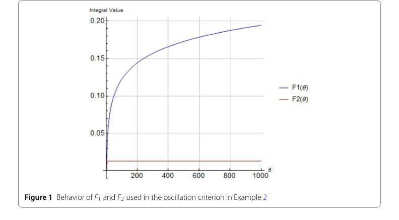 Figure 1. Behavior of F1 and F2 used in the oscillation criterion in Example 2
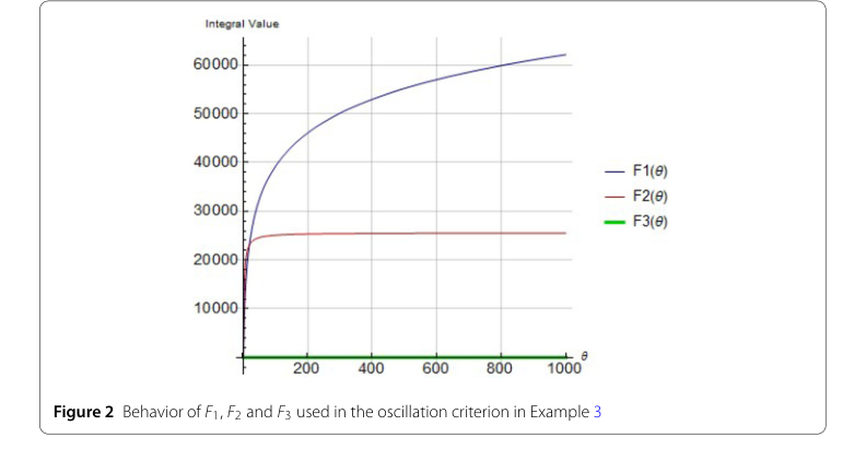 Figure 2. Behavior of F1, F2 and F3 used in the oscillation criterion in Example 3
- Significance of Riccati Transformation: The success of these criteria underscores the power and utility of the Riccati transformation technique, combined with carefully chosen inequalities, as a robust method for analyzing the qualitative behavior of complex differential equations. The derivation of sufficient conditions for the non-existence of positive solutions, which then implies oscillation, is a central and effective mechanism.
In essence, the evidence proves that the authors have not only developed new oscillation criteria but have also demonstrably improved upon existing results, offering a more powerful tool for the qualitative analysis of higher-order neutral nonlinear differential equations.
Limitations & Future Directions
While this paper presents significant advancements in the oscillation theory of higher-order neutral nonlinear differential equations, it's important to acknowledge certain limitations and consider avenues for future development.
Limitations:
- Sufficient Conditions Only: The criteria derived are "sufficient conditions" for oscillation. This means that if the conditions are met, oscillation is guaranteed. However, if the conditions are not met, no conclusion can be drawn about the oscillatory or non-oscillatory nature of the solutions. The absence of "necessary and sufficient" conditions leaves a gap in a complete understanding of the system's behavior.
- Focus on Positive Solutions: The methodology primarily relies on proving the non-existence of eventually positive solutions. While a standard approach (as oscillation implies sign changes, and a symmetric argument often handles eventually negative solutions), it's a specific lens through which to view the problem.
- Canonical Case Specificity: The paper explicitly states its focus on the "canonical case," which typically implies certain integral conditions on the coefficient functions (e.g., $\int_{s_0}^\infty \frac{1}{h^{1/\delta}(\theta)} d\theta = \infty$). This limits the immediate applicability of the results to DEs that do not satisfy this specific condition.
- Complexity of Auxiliary Functions: The effectiveness of the Riccati transformation often depends on the judicious choice of auxiliary functions (like $\psi(\theta)$ in Theorem 5). Finding an optimal or even a suitable $\psi(\theta)$ can be challenging for general cases, potentially limiting the practical application of the theorems.
- Analytical Validation Only: The validation is purely analytical through examples. While rigorous, it doesn't explore the computational aspects or potential numerical instabilities that might arise when trying to apply these criteria in a computational setting for more complex or real-world problems.
Future Directions:
Building upon these findings, several exciting discussion topics and research directions emerge:
- Extension to Non-Canonical Cases: The paper itself proposes studying the oscillation of higher-order DEs (Equation (1)) under the non-canonical condition $\int_{s_0}^\infty \frac{1}{h^{1/\delta}(\theta)} d\theta < \infty$. This is a crucial next step, as many real-world phenomena might fall into this category, requiring different analytical techniques or modifications to the current approach.
- Generalization of Nonlinearities and Delays: The paper also suggests extending the analysis to DEs with more complex nonlinear terms, specifically $\sum_{j=1}^k q_j(s) u^\gamma(\mu_j(s)) = 0$. This opens the door to investigating equations with multiple delays and more intricate functional dependencies, which are common in biological and engineering models.
- Development of Necessary and Sufficient Conditions: A significant advancement would be to derive conditions that are both necessary and sufficient for oscillation, at least for specific subclasses of these NDEs. This would provide a complete characterization of oscillatory behavior, removing the ambiguity of "sufficient only" criteria.
- Numerical and Computational Exploration: Integrating numerical methods could provide a complementary perspective. How do these analytical criteria translate into practical algorithms for predicting oscillation? Can numerical simulations help explore the boundaries of these conditions or identify oscillatory behavior in cases where analytical methods are intractable? This could involve developing software tools that implement these criteria.
- Applications in Specific Fields: Given that DEs model diverse phenomena, a compelling future direction is to identify specific real-world problems (e.g., in population dynamics, control systems, or neural networks) that are governed by these types of higher-order neutral nonlinear DEs. Applying the developed oscillation criteria to these concrete applications could yield valuable insights into system stability, periodic behavior, or chaotic dynamics.
- Robustness and Sensitivity Analysis: How sensitive are the oscillation criteria to small perturbations in the coefficients or delay parameters? Understanding the robustness of these conditions is vital for practical applications where model parameters might be uncertain or subject to noise. This could lead to the development of robust oscillation criteria.
- Exploration of Other Operators: Can the Riccati transformation and inequality techniques be adapted to study oscillation for DEs involving other types of differential operators, such as fractional derivatives, p-Laplacian operators, or even stochastic terms? This would broaden the theoretical framework considerably.
- Qualitative Behavior Beyond Oscillation: While oscillation is a key qualitative property, future work could also explore other behaviors like asymptotic stability, boundedness, or the existence of periodic solutions, using or extending the techniques presented here. This would provide a more holistic understanding of the solution space.
Connections to Other Fields
Mathematical Skeleton
The pure mathematical core of this work involves transforming higher-order neutral differential equations into first-order integral inequalities through a cleaver Riccati-type substitution. The oscillation criteria are then derived by analyzing the asymptotic behavior of these integral inequalities, leveraging specific algebraic inequalities to establish sufficient conditions for the non-existence of eventually positive (non-oscillatory) solutions.
Adjacent Research Areas
Qualitative Theory of Functional Differential Equations
This paper makes a direct contribution to the qualitative theory of functional differential equations, specifically focusing on the oscillatory behavior of neutral types. The Riccati substitution technique, exemplified by the definition of $\Phi(s)$ in equation (20) as $\Phi (s) = \frac{h(s) (y^{(n-1)} (s))^\delta}{\gamma^\delta (\alpha\mu (s))}$, is a fundamental method used to reduce the order of a differential equation and convert it into a first-order differential inequality, which is often more amenable to anaysis. The integral criteria, such as those presented in Theorem 3 (equation (14)) and Theorem 5 (equation (36)), are classic examples of integral averaging techniques widely employed in this field to establish sufficient conditions for the oscillation of solutions.
Grace, S.R., Dzurina, J., Jadlovska, I., Li, T. (2019). On the oscillation of fourth-order delay differential equations. Adv. Differ. Equ. 2019, 118.
Stability Analysis of Time-Delay Systems
The study of neutral differential equations with delay arguments, such as $u(\eta(s))$ and $u(\mu(s))$ in equation (1), has significant implications for the stability analysis of time-delay systems prevalent in control engineering and various physical systems. Oscillatory behavior in such systems often signals instability or undesirable dynamic responses. The conditions derived in this paper for the oscillation of solutions can be directly interpreted as criteria for predicting the onest of instability or sustained oscillations in systems where past states critically influence current dynamics. The rigorous use of inequalities, like Lemma 2 and Lemma 4, to bound solutions and establish their oscillatory nature is a common analytical approach in assessing the stability of complex dynamic systems.
Hale, J. (1977). Theory of Functional Differential Equations. Springer, New York.
Mathematical Modeling in Population Dynamics
Many models in mathematical biology and ecology, particularly those describing population dynamics, inherently incorporate time delays to account for biological processes such as gestation periods, maturation times, or resource regeneration lags. These models frequently take the form of functional differential equations, including neutral types, where the rate of change depends on past states. The oscillation criteria developed in this work provide valuable mathematical tools to predict whether populations modeled by such equations will exhibit stable equilibria or persistent cyclical fluctuations, which are frequently observed phenomena in ecological systems. The analysis of positive solutions and their oscillatory nature directly corresponds to understanding the long-term behavior and stability of biological populations.
Erbe, L.H., Kong, Q., Zhong, B.G. (1995). Oscillation Theory for Functional Differential Equations. Dekker, New York.
[Available Extracted Figures]
- [figure-12-1] Figure 1: Behavior of F1 and F2 used in the oscillation criterion in Example 2
- [figure-14-1] Figure 2: Behavior of F1, F2 and F3 used in the oscillation criterion in Example 3