Compute-Constrained Data Selection

Background & Academic Lineage

The Origin & Academic Lineage

The problem addressed in this paper, "compute-constrained data selection," precisely originates from the practical challenges and substantial resource costs associated with training and finetuning large language models (LLMs). Historically, the concept of data selection itself is not new, dating back to foundational work in machine learning by Hart (1968) and John (1975), where the objective was to create a minimal yet effective dataset from a larger collection. However, with the advent and rapid growth of LLMs, the computational cost of training these models has become immense. Organizations often operate under predetermined, fixed compute budgets—meaning the number of accelerators and their usage hours are allocated in advance. This necessitates an optimal allocation of these resources.

Previous research, such as Hoffmann et al. (2022), began exploring "compute-optimal LLMs" by balancing architectural and training decisions to achieve better perplexity for a given pretraining compute budget. This paper extends that line of inquiry to the post-training finetuning phase of LLMs. While data selection has been recognized as a promising approach to reduce compute requirements during finetuning by reducing dataset size, a critical "pain point" emerged: the efficacy of data selection methods often scales directly with their own computational cost.

The fundamental limitation of previous approaches is that they primarily focused on the effectiveness of data selection in terms of improving model performance or reducing the amount of training data, without adequately considering the computational cost of the selection process itself. Many powerful data selection methods, while effective at identifying high-value data, are themselves computationally intensive. This means that even if a method leads to a smaller, more effective training dataset, the combined cost of selecting the data and then training on it might exceed the total compute budget, or simply be less efficient than a simpler training strategy. In essence, prior methods were not necessarily "compute-optimal" in a holistic sense, as their added cost for selection could outweigh the gains in training efficiency, making real-time or budget-constrained applications impractical. This paper directly tackles this oversight by formalizing data selection within a compute-constrained framework, where both selection and training costs are budgeted.

Intuitive Domain Terms

Here are a few specialized terms from the paper, translated into intuitive analogies for a beginner:

• Finetuning: Imagine you've just learned to play the piano generally, knowing many songs (this is your pre-trained LLM). Now, you're preparing for a specific concert where you only need to play classical pieces. "Finetuning" is like taking your general piano skills and intensely practicing only classical music until you're a virtuoso in that specific genre. You're not learning to play from scratch, but adapting and specializing your existing broad knowledge for a particular, narrower task.

• Compute-Constrained: Think of it like planning a road trip with a strict fuel budget. You want to see as many sights as possible (achieve high performance), but every mile you drive (every computation step) consumes fuel. "Compute-constrained" means you have to be very smart about your route and stops to maximize your sightseeing within that fixed fuel limit, because you can't just fill up the tank whenever you want.

• Data Selection: Picture yourself trying to learn a new language from a massive dictionary. "Data selection" is like having a smart friend who tells you, "Don't memorize the whole dictionary! Focus on these 1,000 most common words and phrases; they'll give you 90% of what you need to communicate effectively." It's about picking the most impactful pieces of information to learn efficiently, rather than trying to process everything.

• Perplexity (PPL): Imagine you're playing a guessing game where you try to predict the next word in a sentence. If the sentence is "The dog barked at the...", and you guess "cat", that's a pretty good guess. If you guess "cloud", that's a surprising, less likely guess. "Perplexity" is a measure of how "surprised" a language model is by a piece of text. A low perplexity means the text is very predictable and fits well with the model's understanding, while a high perplexity means it's unexpected or confusing. In data selection, we might look for data that is just surprising enough to teach the model something new, but not so random that it's unhelpful.

Notation Table

Notation	Description
$D$	The large initial training dataset from which a subset is selected.
$S$	A subset of data points chosen from $D$ for finetuning.
$S^*$	The optimal subset of data points that maximizes performance under constraints.
$T$	The target test dataset used to evaluate the finetuned model's performance.
$V$	The validation set, often used as a proxy for the test set during data selection.
$P(\cdot)$	A function representing the performance of a model on a given dataset.
$T(S)$	A language model that has been trained (finetuned) using the data subset $S$.
$v(x; V)$	A utility function that assigns a relevance score to a single data point $x$ from $D$ based on its relationship to the validation set $V$.
$K$	The total compute budget, typically measured in FLOPs, allocated for both data selection and model training. (Note: In Section 3, $K$ initially denotes maximum data cardinality, but is redefined as compute budget in Section 4, which is the central focus of this paper).
$C_T(S)$	The computational cost incurred when training the model on the selected data subset $S$.
$\sum_{x \in D} C_U(x)$	The total computational cost of computing the utility function for all data points in the original dataset $D$.
$P_0$	The zero-shot performance, representing the model's performance without any additional finetuning or training.
$P$	The upper bound on performance, representing the maximum achievable performance for a given task.
$\lambda$	A parameter that quantifies how efficiently a specific data selection method extracts value from additional compute.

Problem Definition & Constraints

Core Problem Formulation & The Dilemma

The central problem addressed by this paper stems from the practical challenges of finetuning Large Language Models (LLMs) under strict computational budgets.

Input/Current State:
Researchers and practitioners are typically given a large training dataset, $D$, a target test dataset, $T$, and a validation set, $V$. The traditional goal of data selection is to identify an optimal subset of data, $S \subset D$, to train a model $T(S)$ that maximizes performance $P(T; T(S))$ on the test set, subject to a data budget constraint on the size of the subset, $|S| \le K$. This is formally expressed as:
$$ S^* = \arg \max_{S \subset D} P(T; T(S)) \quad \text{subject to} \quad |S| \le K $$
This formulation assumes that the primary bottleneck is the amount of data that can be used for training, and methods often rely on a two-step greedy algorithm: scoring all data points in $D$ using a utility function $v(x; V)$ (a proxy for $P(V; T(\{x\}))$) and then selecting the top $K$ points.

Desired Endpoint (Output/Goal State):
The paper aims to move beyond a data-budget-centric view to a compute-constrained setting. The desired outcome is to determine the optimal allocation of a total compute budget across various aspects of LLM finetuning, including model size, the number of training tokens, and the choice of data selection method. The goal is to find a finetuning strategy that yields the highest possible model performance on a target task, given a fixed and predetermined total computational budget.

Exact Missing Link or Mathematical Gap:
The critical missing link is the explicit consideration of the computational costs associated with both the data selection process itself and the subsequent training on the selected data. The traditional formulation (Equation 1) only constrains the size of the selected dataset, not the compute required to select it or to train on it. This paper bridges this gap by formalizing the problem as a compute-constrained combinatorial optimization problem. The new objective function explicitly incorporates these costs:
$$ S^* = \arg \max_{S \subset D} P(V; T(S)) \quad \text{subject to} \quad C_T(S) + \sum_{x \in D} C_U(x) \le K $$
Here, $K$ now represents the total compute budget (e.g., maximum FLOPs), $C_T(S)$ is the computational cost of training the model on the selected subset $S$, and $\sum_{x \in D} C_U(x)$ is the computational cost of computing the utility function for all data points in the original dataset $D$ to facilitate selection. The sum is over $D$ because, even if only a subset $S$ is chosen, the utility function must typically be computed for all candidate points in $D$ to make an informed selection.

Painful Trade-off or Dilemma:
The core dilemma that has "trapped" previous researchers is the painful trade-off between the efficacy of a data selection method and its computational cost. While more sophisticated data selection methods (e.g., those based on perplexity or gradients) can significantly improve finetuning effectiveness per training step (i.e., achieve better performance with less data), they often incur a substantial computational overhead during the selection phase. This means that a method that is highly effective at identifying valuable data might not be compute-optimal when the total budget is considered, because its selection cost outweighs the benefits it provides in reduced training compute or improved performance. The paper highlights that "even if data selection is effective, it does not a priori imply that it is compute-optimal." A truly compute-optimal method must therefore be both effective at improving training and cheap to compute.

Constraints & Failure Modes

The problem of compute-constrained data selection is inherently difficult due to several harsh, realistic constraints:

1. Predetermined Total Compute Budget: In practical LLM finetuning scenarios, the total compute budget (e.g., number of accelerators, GPU hours) is often fixed and allocated in advance. This imposes a hard computational constraint, meaning any proposed solution must operate within these predefined limits, forcing a careful balance between data selection and training costs.
2. High Computational Cost of LLM Training: Training LLMs, even finetuning, is extremely compute-intensive. Each gradient step consumes significant FLOPs. While data selection aims to reduce the dataset size, the gains from this reduction must be substantial enough to offset any added cost from the selection process itself. This is a fundamental computational constraint.
3. Varying and Significant Costs of Data Selection Methods: Different data selection methods have vastly different computational footprints, which can be substantial:
   • Lexicon-Based (e.g., BM25): These are very cheap, with FLOPs costs approaching 0 (e.g., 1 $\times 10^8$ FLOPs).
   • Embedding-Based: These methods require running an embedding model, incurring moderate costs (e.g., 4.4 $\times 10^{16}$ FLOPs for Embed using a 220M parameter model).
   • Perplexity-Based: These methods require a forward pass of the LLM for each data point to compute perplexity, which is significantly more expensive (e.g., 1.53 $\times 10^{18}$ FLOPs for a 7B model).
   • Gradient-Based (e.g., LESS): These are the most computationally demanding, involving warm-up training and gradient computations, which can be approximately three times the cost of a forward pass (e.g., 8.27 $\times 10^{18}$ FLOPs for a 7B model).
     The wide range of these computational costs means that a method's theoretical effectiveness might be entirely undermined by its practical expense.
4. Scaling Dependencies: The compute-optimal data selection strategy is not static; it changes with the scale of the training model size and the overall compute budget. A method that is compute-optimal for a small model or budget might be suboptimal for a larger one, and vice versa. This necessitates extensive empirical analysis across a wide range of model sizes (7B to 70B parameters in this paper) and budgets, posing a significant data-driven and empirical constraint on understanding the problem.
5. Non-Differentiable Objective (Combinatorial Optimization): The problem of selecting an optimal subset $S$ from $D$ is a combinatorial optimization problem. Directly optimizing the performance $P(T; T(S))$ over all possible subsets is generally intractable, especially when coupled with compute constraints. This mathematical complexity forces reliance on greedy algorithms and approximations, which may not always yield the globally optimal solution.
6. Diminishing Returns: The value of information gained from selecting additional data points often diminishes as more points are explored. This logical constraint means that at some point, the marginal benefit of a more sophisticated (and costly) selection method may not justify its added computational expense. This makes finding the "tipping point" for compute-optimality a key challenge.

Why This Approach

The Inevitability of the Choice

The adoption of a compute-constrained data selection framework was not merely an improvement but a fundamental necessity for practical LLM finetuning. The authors realized that traditional "SOTA" data selection methods, which primarily focus on maximizing model performance given a fixed data budget (e.g., selecting $K$ data points), were inherently insufficient for the real-world challenges of finetuning large language models. The exact moment of this realization is articulated in Section 4, where the paper states that the framework presented in Section 3 (the traditional data selection objective, Equation 1) is "insufficient for the practical challenge of finetuning LLMs." The core issue identified is that LLM finetuning is "often bottlenecked by a computational budget and not a data budget."

This insight highlighted a critical flaw in existing approaches: they failed to account for the computational cost of the data selection process itself. If a method requires extensive compute to identify the "best" subset of data, that cost must be weighed against the gains in training efficiency. Without this compute-aware perspective, even methods that theoretically yield superior data subsets could be rendered impractical or sub-optimal when the total computational budget is limited. Therefore, the shift to a compute-constrained objective, which explicitly budgets for both data selection and training costs, became the only viable solution to address the practical constraints faced by practitioners.

Comparative Superiority

The compute-constrained approach offers qualitative superiority by fundamentally altering the optimization landscape from a data-centric view to a holistic compute-centric one. Beyond simple performance metrics, this method's structural advantage lies in its ability to identify compute-optimal strategies, not just data-optimal ones. It provides a framework to understand the trade-off between the cost of selecting data and the gain in training performance, revealing which methods are truly efficient under a given budget.

For instance, the paper demonstrates that "many powerful data selection methods are almost never compute-optimal, and that cheaper data selection alternatives dominate both from a theoretical and empirical perspective" (Abstract). This is a profound qualitative advantage: it guides practitioners away from blindly adopting methods that perform well on data-centric benchmarks but are prohibitively expensive in terms of FLOPs. The framework inherently handles the high-dimensional noise of real-world compute budgets by providing a clear metric for efficiency. It doesn't directly reduce memory complexity from $O(N^2)$ to $O(N)$, but it enables the selection of methods that are more efficient in terms of FLOPs, thereby optimizing overall resource utilization. The analysis shows that for perplexity and gradient-based data selection to be compute-optimal, the training-to-selection model size ratios need to be 5x and 10x, respectively (Abstract, Section 8), providing a crucial structural insight into when these more complex methods become viable.

Alignment with Constraints

The chosen compute-constrained data selection method perfectly aligns with the problem's harsh requirements by explicitly incorporating the total computational budget as a primary constraint. As inferred from the canonical "Problem Definition & Constraints" section, the central requirement is to optimize model performance under a predetermined, finite compute budget that must cover all computational activities, including data selection and training.

The "marriage" between the problem's requirements and the solution's unique properties is evident in the formalization of the objective function (Equation 2, Section 4):
$$ S^* = \arg \max_{S \subset D} P(V; T(S)) \\ \text{subject to } C_T(S) + \sum_{x \in D} C_U(x) \le K. $$
Here, $K$ represents the total compute budget (e.g., maximum number of FLOPs). The constraint $C_T(S) + \sum_{x \in D} C_U(x) \le K$ directly mandates that the combined cost of training the model on the selected subset $S$ ($C_T(S)$) and the cost of computing the utility function for all data points in the dataset $D$ ($\sum_{x \in D} C_U(x)$) must not exceed the total budget. This formulation directly addresses the two major computational bottlenecks identified in the paper: the cost of training and the cost of data selection utility computation. By optimizing performance within this combined budget, the approach ensures that resource allocation is compute-optimal, directly satisfying the core constraint.

Rejection of Alternatives

The paper does not reject other popular machine learning paradigms like GANs or Diffusion models, as they are outside the scope of data selection. Instead, it critically evaluates and, in many compute-constrained scenarios, effectively "rejects" the unconditional use of more sophisticated and computationally expensive data selection methods in favor of simpler, cheaper alternatives.

The reasoning behind this rejection is rooted in the compute-constrained perspective:
1. FLOP Inefficiency: The paper explicitly states that "powerful data selection methods that use model perplexity or gradient information tend to be FLOP inefficient both from a theoretical and empirical perspective" (Section 2). Methods like Perplexity-Based (PPL) and Gradient-Based (LESS) require significant computational resources for their utility function calculations (Table 1, Table 5).
2. Sub-optimal Performance under Budget: For small and medium compute budgets, the empirical results (e.g., Figure 2, Figure 5 (b)) consistently show that cheaper methods like Lexicon-Based (BM25) and Embedding-Based (Embed) outperform PPL and LESS. This is because the high initial cost of PPL and LESS means that by the time they have selected data, less compute remains for the actual training, leading to worse overall performance within the same total budget. The marginal benefit of using a more sophisticated method often does not outweigh its cost in selecting the data (Section 7).
3. Conditional Viability: While not an outright rejection, the paper implies that these expensive methods are only viable under specific conditions, such as when the training model is significantly larger than the data selection model (e.g., 5x for PPL, 10x for LESS, as per Section 8 and Figures 9, 10). Without these favorable ratios, their high compute cost makes them compute-suboptimal.

In essence, the paper argues that while methods like PPL and LESS might be effective at identifying high-quality data, their computational overhead makes them a poor choice when compute is a strict constraint, unless the scale of the training task is sufficiently large to amortize their selection cost. This is a crucial distinction from simply rejecting them for being ineffective; they are rejected for being inefficient in the context of compute-constrained finetuning.

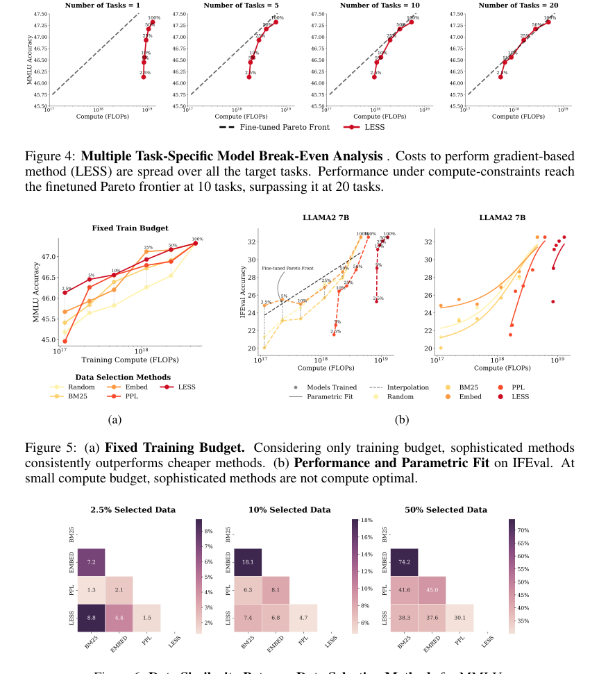Figure 6. Data Similarity Between Data Selection Methods for MMLU

Mathematical & Logical Mechanism

The Master Equation

The paper formalizes the problem of compute-constrained data selection with an objective function that seeks to maximize model performance under a total compute budget. This problem is defined as:

$$ S^* = \arg \max_{S \subset \mathcal{D}} P(\mathcal{V};\mathcal{T}(S)) \\ \text{subject to } C_{\mathcal{T}}(S) + \sum_{x \in \mathcal{D}} C_u(x) \leq K. $$

While this equation defines the problem, the core mathematical engine that powers the analysis and extrapolation in this paper is a parametic model for expected performance, which captures diminishing returns and compute dependence. This model is presented as:

$$ P(k) = (P - P_0) \times \left(1 - \exp\left(-\frac{\lambda C(k)}{C(|\mathcal{D}|)}\right)\right) + P_0 $$

where $C(k)$ is defined as the total cost of training and selection:

$$ C(k) = c \times k + \sum_{x \in \mathcal{D}} C_u(x) $$

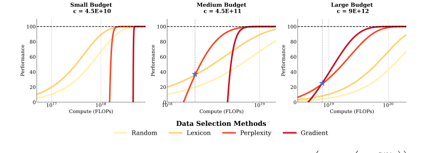Figure 1. Simulation of Performance under Constraints. P(k) = ¯P × ? 1 −exp ? −λ C(k)

Simulation Figure 1 presents a simulation of this performance function across different methods under varying compute constraints. We set $c$ to $\{4.5 \times 10^{10}, 4.5 \times 10^{11}, 9 \times 10^{12}\}$, $k$ to 100M, and utility compute to $\{4.5 \times 10^{10}, 4.5 \times 10^{11}, 9 \times 10^{12}\}$. The parameter $\lambda$ is set to $\{5, 10, 40, 80\}$ for the Random, Lexicon, Perplexity, and Gradient methods, respectively. These settings demonstrate how different data selection methods may become compute-optimal under varying compute budgets. Note that for Medium and Large Budgets, we use a Small-size model for PPL and Gradient.

Term-by-Term Autopsy

Let's dissect the primary parametric performance model, Equation (3), and its auxiliary cost function, $C(k)$, to understand each component's role.

• $P(k)$:

  • Mathematical Definition: The predicted expected performance of the model after training on $k$ selected data points.
  • Physical/Logical Role: This is the output of our model, representing the performance metric (e.g., MMLU accuracy, BBH accuracy) that the paper aims to predict and optimize. It quantifies how well the model performs given a certain number of training data points and the associated compute.
  • Why operators: The overall structure of the equation is designed to model a learning curve, starting from a baseline ($P_0$) and asymptotically approaching an upper bound ($P$) with diminishing returns as compute increases.

• $P$:

  • Mathematical Definition: The upper bound on performance, representing the maximum achievable performance.
  • Physical/Logical Role: This term acts as the ceiling for the model's performance. It signifies the best possible performance the model can reach, typically corresponding to training on the entire dataset or with an infinite compute budget. It defines the maximum potential improvement.
  • Why operators: It is used in the term $(P - P_0)$ to define the total range of potential performance improvement that the exponential growth can cover. It's also added at the end to shift the entire curve to the correct performance scale.

• $P_0$:

  • Mathematical Definition: The zero-shot performance, i.e., the performance of the model without any additional training or finetuning.
  • Physical/Logical Role: This is the baseline performance. It represents the starting point of the learning curve, reflecting the inherent capability of the pre-trained model before any data selection or finetuning is applied.
  • Why operators: It is subtracted from $P$ to define the gain that can be achieved, and then added back at the end to ensure the performance curve starts from this baseline.

• $\lambda$:

  • Mathematical Definition: A parameter controlling how efficiently the method extracts value from additional compute. It is a positive scalar.
  • Physical/Logical Role: This parameter dictates the "steepness" or efficiency of the performance improvement curve. A larger $\lambda$ implies that the method gains performance more rapidly for a given amount of compute, indicating higher compute efficiency.
  • Why operators: It is multiplied by the ratio of current compute to total compute, directly scaling the exponent of the exponential function. This scaling directly controls the rate at which performance approaches the upper bound.

• $C(k)$:

  • Mathematical Definition: The total computational cost (e.g., FLOPs) incurred for selecting $k$ data points and then training the model on that subset.
  • Physical/Logical Role: This term quantifies the total compute budget consumed by the entire process for a given subset size $k$. It's a sum of the cost of training on $k$ points and the fixed cost of utility computation for the full dataset.
  • Why operators: It's a sum because the total cost is composed of two distinct, additive components: the cost of training and the cost of selection.

• $C(|\mathcal{D}|)$:

  • Mathematical Definition: The total computational cost of training on the entire dataset $\mathcal{D}$.
  • Physical/Logical Role: This term serves as a normalization factor for the compute budget. By dividing $C(k)$ by $C(|\mathcal{D}|)$, the exponent becomes a dimensionless ratio representing the fraction of total possible compute utilized. This helps in comparing different methods on a common scale.
  • Why operators: Division by this term normalizes the effective compute, making the exponent dimensionless and allowing the exponential function to model a proportion of the total learning capacity.

• $c$:

  • Mathematical Definition: The fixed-cost of training on a single data point.
  • Physical/Logical Role: This represents the per-data-point computational expense during the training phase. It's a fundamental unit of training cost.
  • Why operators: It is multiplied by $k$ to calculate the total training cost for $k$ data points, assuming a linear relationship between data points and training cost.

• $k$:

  • Mathematical Definition: The number of data points selected for training.
  • Physical/Logical Role: This is the independent variable representing the size of the finetuning dataset. It's the primary factor that practitioners can control to manage training compute.
  • Why operators: Multiplied by $c$ to determine the variable portion of the total compute cost related to training.

• $\sum_{x \in \mathcal{D}} C_u(x)$:

  • Mathematical Definition: The total cost of computing the utility function for all data points $x$ in the full dataset $\mathcal{D}$.
  • Physical/Logical Role: This represents the fixed overhead cost of the data selection process itself. To select a subset, one must first evaluate the utility of all candidate data points in the original dataset. This cost is incurred once, regardless of how many points are ultimately chosen for training.
  • Why operators: It is added to the training cost because it's a necessary, fixed component of the total compute budget for data selection methods.

• $\exp(\cdot)$:

  • Mathematical Definition: The exponential function, $e^x$.
  • Physical/Logical Role: This function is crucial for modeling the diminishing returns characteristic of learning processes. As more compute is invested, the rate of performance improvement naturally slows down, asymptotically approaching the upper bound.
  • Why operators: The negative exponent ensures that as the compute ratio $\frac{\lambda C(k)}{C(|\mathcal{D}|)}$ increases, the term $1 - \exp(-\dots)$ grows from 0 towards 1, creating the desired S-shaped learning curve.

• $\times$, $+$, $-$, $/$, $\leq$:

  • Mathematical Definition: Standard arithmetic operators (multiplication, addition, subtraction, division) and an inequality operator.
  • Physical/Logical Role: These operators combine the various terms in a structured way to represent the complex relationship between compute, data, and performance. Subtraction $(P - P_0)$ defines the range of possible improvement. Multiplication scales this range by the exponential term. Addition shifts the entire curve by $P_0$. Division normalizes the compute. The inequality operator in the objective function defines the compute budget constraint.

Step-by-Step Flow

The parametric model in Equation (3) doesn't process individual data points in the same way a neural network does. Instead, it models the outcome of a data selection and training process based on the number of data points used and the compute consumed. Here's how the lifecycle of the concept of data points (represented by their count $k$) flows through this mathematical engine to predict performance:

1. Input: Number of Data Points ($k$): The process begins with a decision: how many data points, $k$, will be selected for finetuning? This $k$ is the primary input to the performance model.

2. Compute Cost Calculation ($C(k)$):

   • First, the training cost for these $k$ points is determined by multiplying $k$ by $c$, the fixed cost of training on a single data point ($c \times k$). This represents the variable compute cost directly proportional to the size of the selected subset.
   • Next, a fixed overhead cost, $\sum_{x \in \mathcal{D}} C_u(x)$, is added. This represents the compute required to evaluate the utility of all data points in the original dataset $\mathcal{D}$ to enable the selection process, regardless of how many are ultimately chosen.
   • These two components are summed to yield $C(k)$, the total compute cost for both selection and training for the chosen $k$ data points.

3. Compute Normalization: The calculated total compute $C(k)$ is then divided by $C(|\mathcal{D}|)$, the total compute cost if the entire dataset $\mathcal{D}$ were used for training (and its utility computed). This normalization step converts the absolute compute cost into a relative measure, indicating what fraction of the maximum possible compute is being utilized.

4. Efficiency Scaling ($\lambda$): The normalized compute ratio is multiplied by $\lambda$, a parameter representing the efficiency with which a particular data selection method extracts value from compute. This scales the effective compute, influencing how quickly performance improves.

5. Diminishing Returns Transformation: The scaled compute ratio (with a negative sign) becomes the exponent of the exponential function, $1 - \exp(-\frac{\lambda C(k)}{C(|\mathcal{D}|)})$. This is the core mechanism for modeling diminishing returns. Initially, for small compute values, this term grows rapidly, indicating significant performance gains. As compute increases, the rate of growth slows down, reflecting that each additional unit of compute yields smaller incremental performance improvements. This term approaches 1 as compute approaches infinity.

6. Performance Range Scaling: The result from the diminishing returns transformation is multiplied by $(P - P_0)$. This term represents the total potential performance improvement available, from the zero-shot baseline ($P_0$) to the upper bound ($P$). This multiplication scales the diminishing returns curve to fit within the actual performance range.

7. Baseline Offset: Finally, $P_0$ (the zero-shot performance) is added to the scaled improvement. This shifts the entire curve upwards, ensuring that the predicted performance starts from the model's inherent capability before any finetuning.

8. Output: Predicted Performance ($P(k)$): The final value, $P(k)$, is the model's prediction of the expected performance given the initial input of $k$ data points and their associated compute costs. This output is then compared against observed empirical performance.

Optimization Dynamics

The mechanism learns, updates, and converges by fitting the parametric model (Equation 3) to observed empirical data. This is achieved through a non-linear least squares optimization process.

1. Defining the Loss Landscape: The paper defines an objective function to minimize the sum of squared differences between the predicted performance $P(k_i; P_0, P, \lambda)$ and the observed performance $P_{obs,i}$ for various data points $k_i$. This sum of squared errors forms the loss landscape. Due to the exponential term in $P(k)$, this landscape is non-linear and can have complex contours.

   $$ \min_{P_0,P,\lambda} \sum_{i=1}^N (P(k_i; P_0, P, \lambda) - P_{obs,i})^2 $$

2. Parameter Learning: The "learning" in this context refers to finding the optimal values for the model's parameters: $P_0$ (zero-shot performance), $P$ (upper bound performance), and $\lambda$ (compute efficiency). These parameters are not learned iteratively from individual data points like in a neural network, but rather are fitted to the overall performance curve observed across different $k$ values and compute budgets.

3. Optimization Algorithm: The paper employs the Levenberg-Marquardt algorithm for this minimization task. This algorithm is a popular choice for non-linear least squares problems because it effectively combines the robustness of gradient descent (for when parameters are far from the optimum) with the speed of the Gauss-Newton method (for when parameters are close to the optimum). It implicitly uses gradient information (or approximations of the Jacobian matrix) to determine the direction and step size for parameter updates.

4. Iterative Updates: The Levenberg-Marquardt algorithm iteratively updates the parameters $P_0, P, \lambda$ by calculating the gradients of the sum of squared errors with respect to these parameters. It then takes steps in a direction that reduces the error, adjusting the step size based on the local curvature of the loss landscape.

5. Constraints and Initial Guesses: To ensure meaningful and stable parameter estimates, several constraints and initial guesses are applied:

   • Constraints: $P_0 \ge 0$ (performance cannot be negative), $P_0 \le P$ (zero-shot performance cannot exceed the upper bound), and $\lambda \ge 0$ (efficiency cannot be negative, as performance should improve or stay flat with compute).
   • Initial Guesses: The optimization starts with reasonable initial estimates: $P_0^{(0)}$ is set to the observed performance at zero-shot, $P^{(0)}$ is set to the maximum observed performance, and $\lambda^{(0)}$ is set to 1.0. Additionally, $P$ is set slightly above the maximum observed performance by a small buffer $\epsilon = 0.05$ to aid convergence.

6. Convergence: The optimization process continues until the parameters $P_0, P, \lambda$ converge to values that minimize the sum of squared errors, subject to the imposed constraints. At convergence, the fitted parametric model provides the best possible curve that explains the observed performance data, allowing for analysis and extrapolation of compute-performance relationships. The resulting fitted parameters are then used to understand the compute-optimal ratios for different data selection methods.

Results, Limitations & Conclusion

Experimental Design & Baselines

The authors meticulously designed their experiements to rigorously test the hypothesis that compute-constrained data selection necessitates a careful trade-off between the computational cost of selecting data and the cost of training the model. Their core mathematical claim is formalized by the objective function:
$$ S^* = \arg \max_{S \subset D} P(V; T(S)) \quad \text{subject to} \quad C_T(S) + \sum_{x \in D} C_U(x) \le K $$
Here, $P(V; T(S))$ represents the model's performance on a validation set $V$ after training on a selected subset $S$, $C_T(S)$ is the training cost, $C_U(x)$ is the utility computation cost for a data point $x$, and $K$ is the total compute budget in FLOPs. To model the performance, they introduced a parametric function:
$$ P(k) = (P - P_0) \times \left(1 - \exp\left(-\frac{\lambda C(k)}{C(|D|)}\right)\right) + P_0 $$
This function captures diminishing returns, dependence on computational cost, and convergence towards an upper bound, $P$, from a zero-shot performance, $P_0$.

To validate this, they conducted a comprehensive sweep of over 600 training runs, varying compute budgets, model sizes, and data selection methods across three distinct downstream tasks. The "victims" (baseline models) against which their compute-aware approach was tested included:
- Random Selection: A straightforward baseline where data is chosen arbitrarily.
- Lexicon-Based (BM25): A low-cost method relying on statistical properties of text, with an estimated selection cost of $1 \times 10^8$ FLOPs.
- Embedding-Based (Embed): Utilizes a small T5-based dense embedding model to select data points similar to validation data, incurring a selection cost of $4.4 \times 10^{16}$ FLOPs.
- Perplexity-Based (PPL): Evaluates data utility based on model loss (perplexity) using an LLAMA2 model, with a higher selection cost of $1.53 \times 10^{18}$ FLOPs.
- Gradient-Based (LESS): The most compute-intensive method, assessing data influence on model loss through gradient computations, requiring a substantial $8.27 \times 10^{18}$ FLOPs for selection.

The experiments spanned LLAMA2 models (7B, 13B, 70B parameters) and LLAMA3 8B, finetuned using LoRA. The training data budget was varied as a percentage of total tokens (2.5%, 5%, 10%, 25%, 50%, 100%), and compute was allocated either to larger models or more sophisticated data selection. Performance was evaluated on MMLU (5-shot accuracy), BBH (3-shot exact match), and IFEval (0-shot accuracy). The authors then fitted power laws to the FLOP counts to derive finetuned Pareto frontiers for each model size, allowing for a direct comparison of compute efficiency.

What the Evidnece Proves

The empirical evidence strongly supports the paper's central argument: sophisticated data selection methods, while powerful, are often not compute-optimal in a budget-constrained setting. The definitive evidence for this comes from the Pareto frontiers generated across various compute budgets and model sizes.

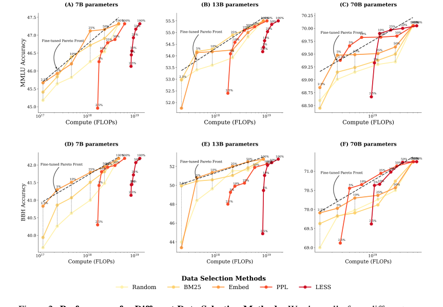Figure 2. Performance for Different Data Selection Methods. We show all of our different runs for a given model size, where each scatter point is the final target task performance of a single run. (A, B, C) show MMLU results across three model sizes, while (D, E, F) present BBH results across three model sizes. For each run, we determine the optimal finetuning strategy—a combination of data selection method and number of finetuning tokens—that achieves the highest performance un- der a particular FLOPs budget. We fit a pareto front in dashed line based on these optimal strategies, which is a line in the linear-log space. At small and medium compute budgets (A, B, D, E), cheaper data selection methods like BM25 and EMBED outperform PPL and LESS, which rely on model information. At larger compute budgets (C, F), however, PPL and LESS become compute-optimal after using 5% of the fine-tuning tokens

For small and medium compute budgets (e.g., with 7B and 13B LLAMA2 models), the cheaper lexicon-based (BM25) and embedding-based (Embed) methods consistently outperformed perplexity-based (PPL) and gradient-based (LESS) methods. This is clearly visible in Figure 2 (A, B, D, E), where the Pareto frontiers for BM25 and Embed lie above those for PPL and LESS at lower FLOPs. The marginal performance gains offered by the more sophisticated methods simply did not justify their significantly higher computational cost for data selection.

However, as the compute budget increased significantly (e.g., with 70B LLAMA2 models), the landscape shifted. For the first time, PPL and LESS became compute-optimal, outperforming BM25 and Embed, particularly after using about 5% of the finetuning tokens (Figure 2 C, F). This demonstrates that while expensive methods are generally not optimal, they can become advantageous when the overall compute budget is very large, allowing their high selection costs to be amortized or when the training model is substantially larger than the selection model.

The parametric fits and subsequent extrapolations provided critcal quantitative insights. For perplexity-based data selection to become compute-optimal, the training model size needed to be approximately 5 times larger than the data selection model (around 35B parameters). For gradient-based data selection, this ratio jumped to approximately 10 times larger (around 70B parameters) (Figures 9 and 10). These ratios provide concrete guidelines for practitioners on when to consider investing in more expensive data selection.

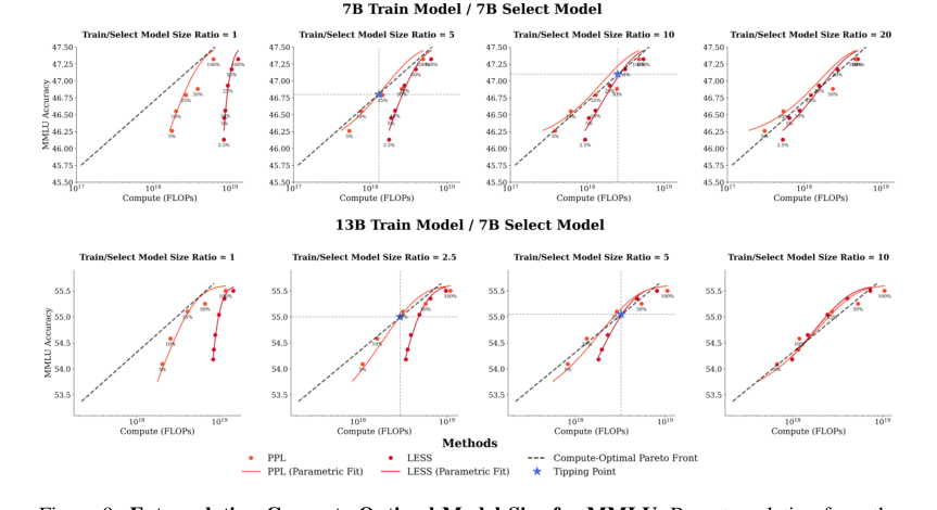Figure 9. Extrapolating Compute-Optimal Model Size for MMLU. By extrapolating from the parametric fits obtained from the 7B and 13B model results for MMLU, we can find the compute- optimal ratio between the training model size and the selector model size required for the perplexity- based and gradient-based method. For perplexity-based data selection, our extrapolation suggests that training model should be larger (5x) than the selector model—around 35B model parameters. For gradient-based data selection to be compute-optimal, our extrapolation suggest that the training model should be significantly larger (10x) than the selector model—specifically, around 70B param- eters in this case

Further, the data similarity analysis (Figure 6) revealed that BM25 and Embed selected highly similar data subsets, which explains their comparable performance. In contrast, LESS selected data with the least resemblance to other methods, suggesting a fundamentally different selection mechanism. This provides a deeper understanding of why certain methods cluster in performance.

Finally, the paper also showed that if the constraint is only on the training budget (ignoring selection cost), gradient-based methods like LESS consistently outperform others (Figure 5a). This highlights the crucial distinction and impact of considering the total compute budget, including data selection. When the cost of gradient computation could be amortized over multiple tasks, LESS also became more competitive, eventually surpassing the finetuned Pareto frontier with 20 tasks (Figure 4).

Limitations & Future Directions

The authors acknowledge several limitations that pave the way for exciting future research. Firstly, the current work focuses on finetuning for a single epoch. Exploring multi-epoch settings where data can be repeated selectively could offer further training speedup, and it would be interesting to see how compute-optimal strategies change in such scenarios.

Secondly, the study fixed most hyperparameters to commonly used values. The effectiveness of finetuning can be highly sensitive to choices like learning rate, dropout, or optimizer. Future work could investigate how hyperparameter tuning interacts with compute-constrained data selection to find more optimal configurations.

Lastly, the paper focused on a specific set of data selection methods based on their compute efficiency. There are other data selection methods, such as classifier-based approaches, that were not covered. Investigating these could provide additional insights into compute-performance trade-offs.

Building on these findings, here are some discussion topics for future development:

• Adaptive Data Selection Frameworks: Can we develop dynamic frameworks that intelligently switch between data selection methods based on the current compute budget, model size, and observed performance? For instance, starting with a cheap method and progressively incorporating more sophisticated ones as the training progresses or as the budget allows for larger training models. This could lead to more robust and universally applicable compute-optimal strategies.
• Novel Compute-Efficient Algorithms: The paper clearly demonstrates that powerful methods like PPL and LESS are often not compute-optimal due to their high selection costs. This calls for a paradigm shift in data selection research: instead of solely focusing on performance, how can we design inherently compute-efficient sophisticated data selection algorithms? This might involve approximations, sampling techniques, or architectural changes that drastically reduce FLOPs for utility computation.
• Beyond Single-Task Amortization: While the paper touched upon amortizing gradient costs over multiple tasks, what about amortizing data selection costs across different models or even different stages of an LLM's lifecycle (e.g., pre-training, instruction-tuning, task-specific finetuning)? Could a shared, compute-intensive data selection step serve multiple downstream applications, making it more cost-effective in a broader ecosystem?
• The Role of Data Quality Metrics: The paper primarily focuses on selecting a subset of existing data. Future work could explore how integrating advanced data quality metrics (e.g., synthetic data generation, adversarial filtering) with compute-constrained selection impacts performance. Can a smaller, meticulously curated dataset, even if selected by a cheaper method, outperform a larger dataset selected by a more expensive method?
• Generalizability Across Diverse LLM Architectures and Modalities: The study primarily used LLAMA2/3 models for instruction-tuning tasks. How do these compute-optimal ratios and method preferences translate to other LLM architectures (e.g., MoE models, smaller specialized models) or different data modalities (e.g., multimodal LLMs, code generation)? Are the identified ratios universal, or do they vary significantly with architectural innovations or task types?

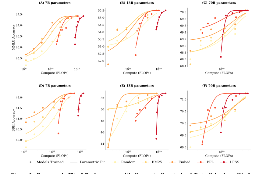Figure 3. Parametric Fit of Performance with Compute-Constrained Data Selection. We fit a parametric model of the performance in Equation (3) and display that as curves to pair with the empirical results as scatter points. (A, B, C) show MMLU results and their parametric fit across three model sizes, while (D, E, F) present BBH results and their parametric fit across three model sizes

Connections to Other Fields

Mathematical Skeleton

The pure mathematical core of this work involves a constrained optimization problem. It aims to maximize a performance function, modeled by a saturating exponential curve, subject to a total compute budget. This budget is composed of a fixed overhead for initial data scoring and a variable cost directly proportional to the amount of data selected for training.

Adjacent Research Areas

Submodular Optimization for Data Selection

The paper explicitly states in Section 3 that the performance function $P(T;T(S))$ is assumed to be "monotonic and submodular, non-increasing marginal utility". This property is central to many data selection strategies, particularly greedy approaches. The problem of selecting a subset of data points to maximize such a submodular function under a resource constraint (like the total compute budget $K$ in Equation 2) is a well-studied area in combinatorial optimization. The paper's formulation extends the basic cardinality-constrained submodular maximization (Equation 1) to a more complex compute budget, where the cost of selection is also considered.
Kirchhoff, K., & Bilmes, J. (2014). Submodularity for data selection in machine translation. Proceedings of the 2014 Conference on Empirical Methods in Natural Language Processing (EMNLP).

Scaling Laws in Deep Learning

The parametic model used to describe the relationship between compute and performance (Equation 3) is a direct application of scaling laws, a prominent area in deep learning research. These laws characterize how various resources (e.g., model size, data size, training FLOPs) impact model performance, often exhibiting power-law or exponential saturation behaviors. The paper leverages this framework to quantify the efficency of different data selection methods and to extrapolate compute-optimal ratios for training-to-selection model sizes.
Kaplan, J., McCandlish, S., Henighan, T., Brown, T. B., Chess, B., Child, R., ... & Amodei, D. (2020). Scaling laws for neural language models. arXiv preprint arXiv:2001.08361.

Budgeted Combinatorial Optimization

The problem can be viewed as a form of budgeted combinatorial optimization, where the goal is to select a subset of items (data points) from a larger collection to maximize a utility (model performance) while adhering to a total budget (compute FLOPs). The budget constraint in Equation 2, which combines a fixed cost for evaluating all items and a variable cost for selected items, is a common structure in problems like the Budgeted Maximum Coverage problem or variants of the Knapsack problem, where items have associated costs and values, and the objective is to maximize total value within a budget. The fixed cost component for utility computation, which is independent of the selected subset size, is a notable feature often occuring in real-world resource allocation scenarios.
Khuller, S., Moss, A., & Naor, J. (1999). The budgeted maximum coverage problem. Information Processing Letters, 70(1), 39-45.