BenchReAD: A systematic benchmark for retinal anomaly detection

Background & Academic Lineage

The Origin & Academic Lineage

The problem of retinal anomaly detection, which this paper addresses, fundamentally emerged from the critical need for efficient and accurate screening of various ocular and systemic diseases. Retinal imaging, utilizing modalities like fundus photography and optical coherence tomography (OCT), is a cornerstone in diagnosing conditions such as diabetic retinopathy, glaucoma, and myopia. Historically, the academic field has recognized the immense potential of automated systems to assist clinicians in this process, especially given the high volume of images and the subtle nature of some anomalies.

However, despite its significance, progress in this domain has been hampered by several fundamental limitations in previous approaches. A major "pain point" has been the absence of a truly comprehensive and publicly available benchmark. Existing benchmarks for medical anomaly detection, particularly those related to retinal images, often suffer from several shortcomings:
1. Limited Scope: They typically rely on single datasets that focus on only one or a few specific diseases, failing to provide a robust and generalizable assessment across the wide spectrum of retinal conditions.
2. Performance Saturation: Some widely used datasets, such as OCT 2017, have become unsuitable as standalone benchmarks because existing models have already achieved near-perfect performance on them, making further evaluation less meaningful.
3. Inadequate Data Utilization: Most prior benchmarks predominantly focus on "one-class supervised" methods, which train only on normal (negative) samples. This approach overlooks the vast amounts of labeled abnormal data and unlabeled data that are readily available in clinical practice, thereby not fully leveraging all available information.
4. Lack of Generalization: Previous experimental setups often lacked rigorous evaluation of how well models generalize to unseen anomaly types, leading to less convincing results in real-world scenarios. The authors were compelled to write this paper to bridge these gaps by introducing a systematic and comprehensive benchmark that addresses these limitations, facilitating fair evaluation and accelerating methodological advancements.

Intuitive Domain Terms

• Retinal Anomaly Detection: Imagine you're looking at a map of a city, and you're trying to find anything that looks out of place – maybe a building that's suddenly much taller than all the others, or a road that abruptly ends. Retinal anomaly detection is like that, but for the back of your eye. It's about using computers to automatically spot unusual or unhealthy features (anomalies) in eye scans that might indicate a disease, like a tiny bleed or a swollen area.
• Fundus Photography: This is essentially a standard, flat photograph of the inside back of your eye, where the retina, optic nerve, and blood vessels are visible. Think of it as taking a regular picture of the "backyard" of your eye. It's a quick and easy way to get a broad overview.
• Optical Coherence Tomography (OCT): If fundus photography is a flat photo, OCT is like a detailed 3D ultrasound, but it uses light instead of sound waves. It creates cross-sectional images of the retina, allowing doctors to see the different layers of tissue and detect subtle changes or fluid buildup that wouldn't be visible in a regular photograph. It's like cutting a cake in half to see all the layers inside.
• One-Class Supervised Methods: Picture teaching a robot what a "normal" apple looks like by showing it thousands of perfect apples. Then, anything that isn't a perfect apple – maybe a bruised apple, a pear, or even a banana – the robot flags as "abnormal." These methods learn only from examples of what's considered normal, and anything that deviates from that learned "normality" is considered an anomaly.
• Disentangled Representations of Abnormalities (DRA): This is a sophisticated way for a computer to learn about diseases. Instead of just seeing a diseased eye as one big "bad" thing, DRA tries to break down the visual information into separate, distinct "signatures" for each type of abnormality. It's like learning to identify different types of cars by focusing on their unique features (e.g., a spoiler for a sports car, a large trunk for a sedan) rather than just the general shape of a car. This helps the model understand what makes each disease unique, even if it hasn't seen that exact combination before.

Notation Table

Notation	Description
$X$	Set of feature vectors extracted from a test image
$M$	Normal Feature Memory, a collection of feature vectors from normal training samples
$x^*$	Most anomalous feature vector from a test image $X$
$m^*$	Closest normal feature vector in $M$ to $x^*$
$||u - v||_2$	Euclidean distance (L2 norm) between vectors $u$ and $v$
$N^M(m^*)$	Set of 'b' features in $M$ that are nearest to $m^*$
$g(X; M)$	Anomaly score derived from comparing test image features with the Normal Feature Memory
$\text{DRA}(X)$	Anomaly score generated by the standalone Disentangled Representation of Abnormalities (DRA) model for image $X$
$f(X; M, \text{DRA})$	Final anomaly score produced by the NFM-DRA model, combining $g(X; M)$ and $\text{DRA}(X)$

Problem Definition & Constraints

Core Problem Formulation & The Dilemma

The core problem addressed by this paper is the lack of a comprehensive, systematic, and robust benchmark for retinal anomaly detection that accurately reflects real-world clinical challenges and facilitates the development of generalizable methodologies.

Starting Point (Input/Current State):
Currently, retinal anomaly detection is a critical task for screening various ocular and systemic diseases using imaging modalities like fundus photography and optical coherence tomography (OCT). However, the field is hindered by several limitations in existing benchmarks and evaluation practices:
1. Limited Anomaly Diversity: Previous work has been constrained by using a "limited and overly simplistic set of anomaly types" in their datasets.
2. Performance Saturation: Test sets in widely used benchmarks, such as the OCT 2017 dataset, are "nearly saturated," meaning current models achieve near-perfect scores, making it difficult to discern true progress or evaluate new methods effectively.
3. Poor Generalization Evaluation: There is a "lack of generalization evaluation," leading to "less convincing experimental setups" that do not adequately assess how models perform on novel, previously unseen anomalies.
4. Supervision Bias: Most existing benchmarks predominantly focus on "one-class supervised approaches" (training only with normal/negative samples), overlooking the "vast amounts of labeled abnormal data and unlabeled data that are commonly available in clinical practice."

Desired Endpoint (Output/Goal State):
The paper aims to establish "BenchReAD," a new benchmark that serves as a "systematic and comprehensive" framework for retinal anomaly detection. This benchmark is designed to:
1. Enhance Data Diversity: Incorporate "notably larger datasets with a more diverse range of anomaly categories" including both seen (present in training) and unseen (absent from training) anomalies, ensuring a rigorous assessment of generalizability.

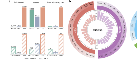Figure 1. (a) Comparison among widely used datasets for retinal anomaly detection (AP- TOS [15], LAG [19], OCT 2017 [16], and RESC [13]) and our BenchReAD. (b) Overview of the test datasets included in the proposed benchmark

1. Systematize Methodology Evaluation: Categorize and benchmark anomaly detection approaches across four supervision levels: unsupervised, one-class supervised, semi-supervised, and fully supervised methods.
2. Improve Robustness to Unseen Anomalies: Address the critical issue where state-of-the-art fully supervised methods, like Disentangled Representations of Abnormalities (DRA), achieve high performance on seen anomalies but suffer "significant drops in performance when encountering certain unseen anomalies." The goal is to develop a more "powerful and stable approach" (NFM-DRA) that mitigates this degradation.
3. Promote Comprehensive Evaluation Metrics: Inspire a "rethinking of evaluation protocols" by drawing "more attention to threshold-dependent metrics" (like F1 scores, specificity, and sensitivity) in addition to threshold-independent ones (like AUC), which are crucial for real-world clinical deployment.

Exact Missing Link or Mathematical Gap:
The exact missing link is a robust mechanism within anomaly detection models, particularly fully supervised ones, to effectively leverage information about "normality" to identify novel, unseen anomalies, rather than solely relying on learned features of seen abnormalities. Mathematically, existing fully supervised models (like DRA) learn a mapping $f_{DRA}(X)$ that distinguishes between known normal and abnormal patterns. The gap is that this mapping, while effective for seen anomalies, does not inherently generalize well to anomalies it has never encountered. The paper proposes to bridge this by introducing a "Normal Feature Memory" ($M$) and integrating its comparison with test image features ($X$) into the anomaly scoring. This is represented by the anomaly score $g(X; M)$ (Equation 2) and its combination with DRA's score in the final anomaly score $f(X; M, DRA)$ (Equation 3). This integration provides a mathematical pathway to explicitly model deviations from learned normal features, thereby enhancing robustness to unseen anomalies.

Painful Trade-off or Dilemma:
The central dilemma that has "trapped previous researchers" is the trade-off between achieving high detection performance on known anomaly types and maintaining robustness/generalizability to unseen anomaly types.
* Fully supervised methods (e.g., DRA) excel at distinguishing between normal and seen abnormal samples because they are trained on both. They learn specific features of these known anomalies, leading to "the best performance" and high AUCs on seen categories. However, this reliance on specific abnormal features makes them brittle; when they encounter an anomaly type not present in their training data (an unseen anomaly), their performance "suffers from a significant drop." They struggle to generalize beyond what they have explicitly learned.
* One-class supervised methods (e.g., PatchCore), conversely, are trained only on normal samples. They learn the distribution of normality and identify anything deviating from it as "abnormal." This approach inherently offers "greater robustness" to unseen anomalies because it doesn't rely on prior knowledge of specific abnormal features. However, their overall performance, especially on seen anomalies, might not always match the peak performance of fully supervised methods.

The dilemma is how to combine the high discriminative power of fully supervised learning for seen anomalies with the inherent generalization capability of normality-modeling for unseen anomalies, without sacrificing either.

Constraints & Failure Modes

The problem of retinal anomaly detection, particularly in the context of creating a robust benchmark, is constrained by several harsh, realistic walls:

• Data-Driven Constraints:

  • Limited Anomaly Type Diversity in Existing Datasets: Previous benchmarks suffered from "a limited and overly simplistic set of anomaly types," which restricted the scope of evaluation and model development. This makes it difficult to assess true generalization.
  • Performance Saturation on Older Benchmarks: Datasets like OCT 2017 have become "unsuitable as a standalone benchmark because of performance saturation." This means models achieve near-perfect scores, making it impossible to differentiate between truly advanced methods and those that merely overfit to the specific, limited anomalies in the dataset.
  • Lack of Generalization Evaluation: A significant constraint is the absence of robust evaluation protocols for generalization, especially to unseen anomalies. This leads to "less convincing experimental setups" that don't reflect real-world clinical scenarios where novel pathologies can emerge.
  • Imbalance in Supervision Paradigms: Existing benchmarks predominantly focused on one-class supervised methods, overlooking the potential of "vast amounts of labeled abnormal data and unlabeled data" available in clinical practice. This limits the exploration of more powerful, data-rich approaches.
  • Need for Threshold-Dependent Metrics: Most anomaly detection evaluations rely on threshold-independent metrics (e.g., AUC), which "limits the evaluation of their readiness for real-world deployment." Clinical settings require specific operating points, making threshold-dependent metrics (F1 score, specificity, sensitivity) crucial but often neglected in benchmarks.

• Computational Constraints:

  • Hardware Memory Limits: The proposed NFM-DRA method, inspired by memory bank mechanisms, involves constructing a "Normal Feature Memory" ($M$) to store features of normal samples. For large datasets, storing these features can be substantial and potentially hit "hardware memory limits," as implied by the mention of experiments being performed on a "single NVIDIA RTX 3090 GPU." This limits the scale and complexity of the memory bank.
  • Computational Cost of Benchmarking: Systematically evaluating multiple anomaly detection methods across various supervision levels and diverse, large datasets (fundus photography and OCT) is computationally intensive. Training and evaluating numerous models with grid search for optimal hyperparameters (learning rate, epochs) requires significant computational resources and time.

• Physical Constraints (Implicit):

  • Variability of Retinal Anomalies: Retinal diseases manifest with immense variability in appearance, size, and location. This inherent biological complexity makes it "insanely difficult" for models to learn a universal representation of "abnormality" that generalizes to all possible conditions, especially those not encountered during training.
  • Imaging Modality Specifics: The benchmark must account for the distinct characteristics and challenges of two different imaging modalities: fundus photography and OCT. Each modality captures different aspects of retinal health, requiring models to be robust across these variations.

Why This Approach

The Inevitability of the Choice

The adoption of NFM-DRA wasn't a pre-ordained choice from the outset, but rather an evolution driven by a critical realization regarding the limitations of even the best existing methods. The authors' extensive benchmarking revealed that the fully supervised approach, Disentangled Representations of Abnormalities (DRA), consistently achieved the highest overall performance among all evaluated methods. This was a significant finding, as DRA leveraged both normal and abnormal labeled data, which is often available in medical imaging but overlooked by traditional one-class supervised anomaly detection.

However, the "exact moment" of insufficiency for DRA, and by extension, other SOTA methods, became apparent when evaluating performance on unseen anomalies. The paper explicitly states that while DRA performed exceptionally well on seen anomalies (those present in the training set), it suffered from "significant drops in effectiveness when encountering certain unseen anomalies." This instability, particularly for categories like Macular Hole (MH), Optic Disc Edema (ODE), Retinoschisis (RS), and Central Retinal Vein Occlusion (CRVO) in the RIADD and JSIEC datasets, highlighted a crucial gap. Traditional methods, including DRA, were not robust enough to generalize to novel, previously unencountered pathological conditions, which is a harsh reality in clinical practice. This vulnerability to unseen anomalies made DRA, despite its overall superiority, an incomplete solution. The need for a more stable and generalizable approach, especially for rare or novel conditions, became undeniable.

Comparative Superiority

NFM-DRA's qualitative superiority stems directly from its structural innovation designed to overcome DRA's Achilles' heel: its lack of robustness to unseen anomalies. While DRA excels by learning disentangled representations of abnormalities, its predictions tend to over-rely on features of previously seen abnormal samples. This makes it brittle when confronted with novel anomaly types.

The proposed NFM-DRA addresses this by integrating a Normal Feature Memory ($M$). This memory bank stores representative features of normal samples. The core structural advantage is that instead of solely relying on learned abnormal patterns, NFM-DRA explicitly models "normality." When a test image feature $X$ is presented, the model not only uses DRA's prediction but also computes an anomaly score $g(X; M)$ based on its similarity to the stored normal features. Specifically, it finds the representative feature $x^*$ from $X$ and its closest feature $m^*$ from $M$ using:

$$x^*, m^* = \arg \max_{x \in X} \arg \min_{m \in M} \|x - m\|_2$$

The anomaly score $g(X; M)$ is then calculated as:

$$g (X; M) = \left(1 - \frac{\exp (\|x^* - m^* \|_2)}{\sum_{m \in N^M(m^*)} \exp \|x^* - m\|_2}\right) \|x^* - m^*\|_2$$

The final anomaly score $f(X; M, DRA)$ is a combination of this memory-based score and DRA's original score:

$$f (X; M, DRA) = \frac{1}{2} [g (X; M) + DRA (X)]$$

This hybrid approach provides a qualitative strength that goes beyond simple performance metrics. It ensures that even if an unseen anomaly doesn't perfectly match any previously learned abnormal features, its deviation from the explicitly modeled normal feature space will still be detected. This dual mechanism provides a more stable and robust detection capability, particularly for anomalies that are rare or novel, without sacrificing the high performance DRA achieves on seen anomalies. The paper does not discuss improvements in high-dimensional noise handling or memory complexity reduction in the context of NFM-DRA.

Alignment with Constraints

The chosen NFM-DRA method perfectly aligns with the critical constraints identified in the problem definition, particularly the need for robust generalization to diverse and unseen anomaly types. The primary limitations of previous retinal anomaly detection work included:

1. Limited and simplistic anomaly types: Existing benchmarks often focused on a narrow range of diseases.
2. Performance saturation on test sets: Many methods achieved near-perfect scores on older, less diverse datasets, making robust evaluation difficult.
3. Lack of generalization evaluation: Methods struggled when encountering unseen anomalies.
4. Over-reliance on one-class supervised methods: These methods ignored valuable labeled abnormal data available in clinical practice.

The proposed NFM-DRA directly addresses the third and most challenging constraint: the lack of generalization to unseen anomalies. While the underlying DRA model (a fully supervised approach) already tackles constraint #4 by utilizing both normal and abnormal labeled data, its weakness on unseen anomalies was a major hurdle. NFM-DRA's integration of a Normal Feature Memory is the "marriage" between this harsh requirement for robustness against novel pathologies and the solution's unique property of explicitly modeling normality. By comparing test images against a learned "normal" feature space, NFM-DRA becomes less dependent on having seen every possible anomaly type during training. This makes it inherently more robust to the diverse and often unpredictable nature of retinal diseases, thereby enhancing its generalization capabilities. The benchmark itself, BenchReAD, addresses the first two constraints by providing a more comprehensive and diverse set of anomaly types and larger datasets to prevent saturation. NFM-DRA then provides a method that can effectively operate within this more rigorous evaluation framework.

Rejection of Alternatives

The paper implicitly, and in some cases explicitly, rejects other popular approaches because of their comparative limitations, particularly concerning robustness to unseen anomalies. The extensive benchmarking process itself serves as the primary mechanism for this rejection.

The authors systematically categorize and evaluate methods across four supervision levels: Unsupervised (e.g., Soft-Patch), One-class supervised (e.g., EDC, SimpleNet, PatchCore), Semi-supervised (e.g., DDAD-ASR), and Fully supervised (DRA).

• Unsupervised and Semi-supervised Methods: These methods generally lagged behind DRA and PatchCore in overall performance (Figure 2, Section 3.1). While they might offer some generalization by not relying on abnormal labels, their overall detection capability was inferior.
• One-class Supervised Methods (e.g., PatchCore): PatchCore, a memory bank-based method, showed "greater robustness for unseen anomalies" and ranked second in overall performance. This indicates that memory-based approaches have an inherent advantage in handling unseen data by modeling normality. However, PatchCore did not achieve the overall highest performance that DRA did on seen anomalies.
• Fully Supervised DRA (without NFM): This was identified as the best-performing approach overall, achieving "notably high AUC values with narrow confidence intervals" across most datasets. However, its critical flaw was its "significant drop in effectiveness when encountering certain unseen anomalies." The paper highlights specific instances where DRA performed "notably weaker" or even "the worst among all comparative methods" on certain unseen categories (e.g., MH, ODE, RS, CRVO, BF w/o PDR). This unstable performance on unseen anomalies was the direct reason for its rejection as a standalone, sufficiently robust solution.

Therefore, the rejection of alternatives was not a blanket dismissal of entire paradigms (like GANs or Diffusion models, which are not explicitly benchmarked by name but fall under the broader categories of anomaly detection methods). Instead, it was a data-driven conclusion that while DRA offered the best overall performance, its specific vulnerability to unseen anomalies necessitated an enhancement. NFM-DRA was thus proposed as an improvement upon the best existing method, rather than a completely new paradigm, to specifically address this critical robustness issue.

Mathematical & Logical Mechanism

The Master Equation

The core of the proposed NFM-DRA (Normal Feature Memory-Disentangled Representation of Abnormalities) mechanism is a three-part mathematical engine. It first identifies the most anomalous feature within a test image relative to a memory of normal features, then computes a memory-based anomaly score, and finally combines this with the score from a pre-trained DRA model.

The first crucial step involves finding the most representative anomalous feature $x^*$ from a test image's feature set $X$ and its closest normal counterpart $m^*$ from the Normal Feature Memory $M$:

$$x^*, m^* = \underset{x \in X}{\arg \max} \underset{m \in M}{\arg \min} ||x - m||_2 \quad (1)$$

Once $x^*$ and $m^*$ are identified, the memory-based anomaly score $g(X; M)$ is computed as:

$$g(X; M) = \left(1 - \frac{\exp(||x^* - m^*||_2)}{\sum_{m \in N^M(m^*)} \exp(||x^* - m||_2)}\right) \cdot ||x^* - m^*||_2 \quad (2)$$

Finally, the NFM-DRA model integrates this memory-based score with the output of the standalone DRA model to produce the final anomaly score $f(X; M, \text{DRA})$:

$$f(X; M, \text{DRA}) = \frac{1}{2} [g(X; M) + \text{DRA}(X)] \quad (3)$$

Term-by-Term Autopsy

Let's dissect these equations to understand each component's role:

Equation (1): Identifying the Most Anomalous Feature

• $X$: This represents the set of feature vectors extracted from a given test image. Its mathematical definition is a collection of high-dimensional vectors. Its logical role is to provide a comprehensive representation of the test image, allowing for localized anomaly detection. The author uses a set because an image typically yields multiple feature patches or embeddings.
• $M$: This is the Normal Feature Memory, a collection of feature vectors derived from purely normal (non-anomalous) training samples. Mathematically, it's a set of feature vectors, $M = \{m_1, m_2, \dots, m_k\}$. Its physical/logical role is to encapsulate the "normality" distribution. By storing features of normal samples, it provides a reference against which new samples can be compared to gauge their deviation from normal.
• $x \in X$: A single feature vector from the test image's feature set.
• $m \in M$: A single feature vector from the Normal Feature Memory.
• $||x - m||_2$: This is the Euclidean distance (L2 norm) between a feature $x$ from the test image and a feature $m$ from the normal memory. Mathematically, for two vectors $u$ and $v$, $||u - v||_2 = \sqrt{\sum_i (u_i - v_i)^2}$. Its logical role is to quantify the dissimilarity between a test feature and a normal feature. A smaller distance implies greater similarity. The L2 norm is chosen because it's a standard, intuitive measure of distance in a continuous feature space, penalizing larger deviations more significantly than, say, the L1 norm.
• $\underset{m \in M}{\arg \min} ||x - m||_2$: This operator finds the feature $m^*$ in the Normal Feature Memory $M$ that is closest (most similar) to a given feature $x$ from the test image. Its logical role is to identify the "best normal match" for any given test feature.
• $\underset{x \in X}{\arg \max} (\dots)$: This operator then searches through all features $x$ in the test image's feature set $X$ and selects the $x^*$ for which its minimum distance to any normal feature (found by the $\arg \min$ operation) is the largest. Its logical role is to pinpoint the specific part of the test image (represented by $x^*$) that is most anomalous or least similar to anything seen in the normal memory. This is a clever way to focus on the strongest anomaly signal within an image.

Equation (2): Computing the Memory-Based Anomaly Score

• $g(X; M)$: This is the anomaly score derived purely from the comparison of the test image features with the Normal Feature Memory. Its logical role is to provide a quantitative measure of how "abnormal" the test image is, specifically leveraging the learned normal feature distribution.
• $\exp(\cdot)$: The exponential function, $e^z$. Its mathematical role is to transform distances into positive, non-linear values, amplifying larger distances more significantly. This helps to make the distinction between "slightly anomalous" and "very anomalous" more pronounced.
• $N^M(m^*)$: This denotes a set of 'b' features in $M$ that are nearest to $m^*$. The paper explicitly states this. Its logical role is to define a local neighborhood around the closest normal feature. This allows the model to assess the anomaly of $x^*$ not just against its single closest normal feature, but also against the local density of normal features.
• $\sum_{m \in N^M(m^*)} \exp(||x^* - m||_2)$: This is the sum of exponentials of distances between $x^*$ and all features in the local neighborhood $N^M(m^*)$. Its logical role is to act as a local normalization factor, similar to the denominator in a softmax function. It provides a measure of the overall "proximity" of $x^*$ to the local cluster of normal features around $m^*$.
• $\frac{\exp(||x^* - m^*||_2)}{\sum_{m \in N^M(m^*)} \exp(||x^* - m||_2)}$: This fraction represents the normalized "similarity" or "proximity" of $x^*$ to its single closest normal feature $m^*$, relative to its proximity to a small group of normal features around $m^*$. If $x^*$ is very close to $m^*$ and also close to its neighbors, this value will be high. If $x^*$ is far from $m^*$ (and its neighbors), this value will be low.
• $1 - (\dots)$: This subtraction inverts the proximity measure. If $x^*$ is very similar to normal features (high proximity), this term will be small. If $x^*$ is very dissimilar (low proximity), this term will be large. This effectively converts a "similarity" score into an "anomaly" score, where higher values indicate greater anomaly.
• $\cdot ||x^* - m^*||_2$: This term multiplies the inverted proximity by the raw Euclidean distance between $x^*$ and $m^*$. Its logical role is to scale the anomaly score. If $x^*$ is far from $m^*$, both the inverted proximity term and the raw distance will be large, resulting in a significantly higher anomaly score. This ensures that the magnitude of the deviation is directly incorporated into the final memory-based score, not just its relative position within the normal feature space. The multiplication here ensures that both the relative "strangeness" and the absolute "distance" contribute to the score.

Equation (3): Combining Scores for Final Anomaly Detection

• $f(X; M, \text{DRA})$: This is the final anomaly score produced by the NFM-DRA model. Its logical role is to provide a comprehensive and robust measure of anomaly by combining insights from both the memory-based approach and the supervised DRA model.
• $\text{DRA}(X)$: This represents the anomaly score generated by the standalone Disentangled Representation of Abnormalities (DRA) model for the test image $X$. The DRA model is a fully supervised approach that learns to disentangle normal and abnormal features. Its logical role is to provide a strong, discriminative anomaly score based on direct supervised learning.
• $\frac{1}{2} [\dots]$: This is a simple arithmetic mean (average) of the two anomaly scores, $g(X; M)$ and $\text{DRA}(X)$. Its logical role is to combine the strengths of both mechanisms. The memory-based score ($g(X; M)$) provides robustness against unseen anomalies by explicitly modeling normality, while the DRA score provides high performance on seen anomalies due to its supervised nature. Averaging them provides a balanced and more stable final prediction. Addition (and subsequent division by 2) is used here because it's a straightforward way to combine two independent scores, giving equal weight to each. This avoids potential issues with multiplication, such as one score dominating or nullifying the other if it's very small.

Step-by-Step Flow

Imagine a single abstract retinal image, let's call it "Image A," entering the NFM-DRA system. Here's its journey:

1. Feature Extraction: First, Image A is fed into a feature extractor (likely a pre-trained deep neural network, though the paper doesn't detail this specific component). This process transforms Image A into a set of high-dimensional feature vectors, $X = \{x_1, x_2, \dots, x_p\}$, representing different regions or aspects of the image. Think of this as Image A being broken down into many small, descriptive pieces.

2. Memory Comparison (Equation 1):

   • For each feature vector $x_i$ in $X$, the system searches through the entire Normal Feature Memory $M$. It calculates the Euclidean distance ($||x_i - m||_2$) between $x_i$ and every single normal feature $m$ stored in $M$.
   • For each $x_i$, it identifies its closest normal feature $m_i^*$ from $M$. This is the $\underset{m \in M}{\arg \min} ||x_i - m||_2$ step.
   • Next, the system compares all these minimum distances. It picks out the feature $x^*$ from $X$ that had the largest minimum distance to any normal feature. This $x^*$ is considered the "most anomalous" part of Image A. The corresponding closest normal feature to this $x^*$ is denoted $m^*$. This completes Equation (1), giving us the specific $x^*$ and $m^*$ that will drive the memory-based anomaly score.

3. Memory-Based Anomaly Score Calculation (Equation 2):

   • Using the identified $x^*$ and $m^*$, the system calculates their raw Euclidean distance, $||x^* - m^*||_2$.
   • It then identifies a small neighborhood, $N^M(m^*)$, of 'b' normal features in $M$ that are closest to $m^*$.
   • The system computes the exponential of the distance between $x^*$ and $m^*$, $\exp(||x^* - m^*||_2)$.
   • Simultaneously, it computes the sum of exponentials of distances between $x^*$ and each feature in the neighborhood $N^M(m^*)$, $\sum_{m \in N^M(m^*)} \exp(||x^* - m||_2)$.
   • These two exponential terms are used to form a ratio, which is then subtracted from 1. This gives a "relative anomaly" score.
   • Finally, this relative anomaly score is multiplied by the raw distance $||x^* - m^*||_2$ to get the final memory-based anomaly score, $g(X; M)$. This score quantifies how "strange" $x^*$ is, both absolutely and relative to its normal surroundings in the feature space.

4. DRA Model Score: In parallel, Image A is also fed into the pre-trained DRA model. The DRA model processes Image A and outputs its own anomaly score, $\text{DRA}(X)$. This score reflects the DRA model's assessment of anomaly based on its supervised training.

5. Final Score Combination (Equation 3): The two anomaly scores, $g(X; M)$ and $\text{DRA}(X)$, are then simply added together and divided by two. This averaging step produces the final, robust anomaly score $f(X; M, \text{DRA})$ for Image A. A higher $f(X; M, \text{DRA})$ indicates a greater likelihood that Image A contains an anomaly.

This entire process is like a two-pronged inspection: one inspector (the memory) checks for deviations from learned normality, while another (DRA) checks for patterns it was explicitly taught to recognize as abnormal. Their combined judgment forms the final decision.

Optimization Dynamics

The NFM-DRA mechanism itself, as described by equations (1), (2), and (3), is primarily a scoring function rather than an iteratively optimized model during the anomaly detection phase. Its "learning" and "updating" happen in its constituent parts:

1. Normal Feature Memory ($M$) Construction: The paper states that the Normal Feature Memory $M$ is "constructed... to store features of normal samples." This implies a one-time, pre-processing step. During training, normal images are passed through a feature extractor, and their resulting feature vectors are collected and stored in $M$. The paper doesn't specify any iterative update rules for $M$ itself during the anomaly detection process. It's a static reference bank once built. The "learning" here is in what features are chosen to represent normality and how they are extracted, which depends on the underlying feature extractor's training.

2. DRA Model Training: The DRA (Disentangled Representation of Abnormalities) model is a "fully supervised approach." This means it undergoes a standard supervised learning process. It would be trained on a dataset containing both labeled normal and abnormal images, using a loss function (e.g., cross-entropy loss for classification, or a more complex loss for disentanglement) and an optimization algorithm like stochastic gradient descent (SGD) or Adam. During this training, the DRA model's internal parameters (weights and biases of its neural network layers) are iteratively adjusted to minimize its loss function, thereby learning to effectively distinguish between normal and abnormal features. The loss landscape for DRA would be shaped by its specific architecture and loss function, guiding the gradients towards optimal parameters.

3. NFM-DRA's Role: The NFM-DRA mechanism combines the output of the pre-trained DRA model with the scores derived from the pre-constructed Normal Feature Memory. It doesn't have its own iterative learning or gradient-based updates during inference. Instead, its "optimization" is in its design: by averaging the two scores, it aims to mitigate the limitations of each individual component. DRA might struggle with unseen anomalies because it's only seen specific abnormal patterns during training. The memory-based component, by focusing on deviations from normality, provides a more generalizable signal for novel anomalies. The simple arithmetic mean acts as a robust fusion strategy, balancing the strengths of both. This design choice is an "optimization" in the sense of creating a more stable and powerful anomaly detection system, rather than an iterative parameter update. The paper highlights that this combination "mitigates the performance degradation" and leads to a "more powerful and stable approach," which is the desired outcome of this logical mechanism.

Results, Limitations & Conclusion

Experimental Design & Baselines

To rigorously validate their claims and establish a comprehensive benchmark, the authors architected BenchReAD to encompass two widely used retinal imaging modalities: fundus photography and optical coherence tomography (OCT). A crucial aspect of their experimental design was the inclusion of both seen (anomaly types present in the training data) and unseen (anomaly types absent from the training data) anomalies within the test sets. This setup was specifically designed to ruthlessly test the generalizability and robustness of anomaly detection models, particularly against novel, clinically relevant conditions.

The "victims" (baseline models) against which the proposed NFM-DRA was benchmarked represent a diverse spectrum of anomaly detection methodologies, categorized by their supervision levels:
* Unsupervised methods: Represented by Soft-Patch, these models operate without any labeled data, relying solely on the inherent structure of the entire dataset (normal, abnormal, and unlabeled).
* One-class supervised methods: This category included EDC, SimpleNet, and PatchCore. These models are trained exclusively on normal images, learning to identify deviations from normality as anomalies. PatchCore, in particular, utilizes a memory bank mechanism, which proved to be a strong baseline for robustness.
* Semi-supervised methods: DDAD-ASR was the representative here, extending one-class supervised approaches by incorporating additional unlabeled data during training.
* Fully supervised methods: DRA (Disentangled Representations of Abnormalities) was the primary baseline in this category. These models leverage both labeled normal and abnormal images to detect anomalies, aiming for high performance on both seen and unseen types.

The training data itself was meticulously partitioned, with one-third designated as labeled and two-thirds as unlabeled, allowing for a fair evaluation of methods across these different supervision paradigms. Performance was primarily measured using Area Under the Receiver Operating Characteristic curve (AUC) for threshold-independent evaluation, complemented by F1 scores, specificity, and sensitivity for threshold-dependent assessment, which is vital for clinical applicability. All experiments were conducted using PyTorch, with optimal hyperparameters identified via grid search on validation sets, and run on a single NVIDIA RTX 3090 GPU, ensuring a consistent and reproducible experimental environment.

What the Evidence Proves

The extensive benchmarking provided definitive, undeniable evidence regarding the strengths and weaknesses of current retinal anomaly detection approaches, and the efficacy of the proposed NFM-DRA.

Firstly, the fully supervised DRA model consistently demonstrated superior overall performance, achieving the highest AUCs across four out of five test sets (RIADD, OCT 2017, OCTDL, and OCTID), often with impressively narrow 95% confidence intervals (Figure 2). This proved that when sufficient labeled abnormal data is available, a model designed to disentangle representations of abnormalities can be exceptionally effective at distinguishing normal from abnormal retinal images.

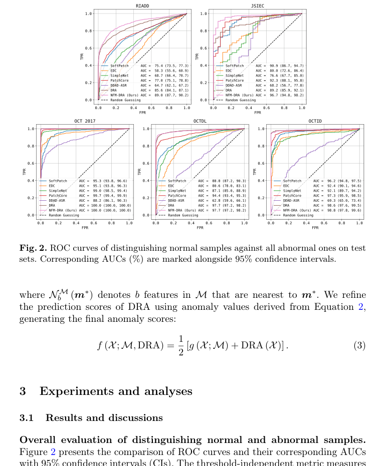Figure 2. ROC curves of distinguishing normal samples against all abnormal ones on test sets. Corresponding AUCs (%) are marked alongside 95% confidence intervals

However, the critical insight emerged when evaluating performance on unseen anomaly categories. While DRA excelled on seen anomalies, its effectiveness suffered a significant drop when encountering certain unseen anomalies. For instance, on the RIADD dataset, DRA's performance was notably weaker for categories like Macular Hole (MH), Optic Disc Edema (ODE), Retinoschisis (RS), and Choroidal Rupture Syndrome (CRS). A similar trend was observed on the JSIEC dataset, where DRA underperformed on unseen anomalies such as Branch Retinal Vein Occlusion (BRVO) and Blur Fundus without PDR (BF w/o PDR), even performing the worst among all comparative methods for the latter (Figure 3, Table 1). This stark contrast was the hard evidence that DRA, despite its overall prowess, lacked the necessary robustness for real-world scenarios where novel anomalies are inevitable.

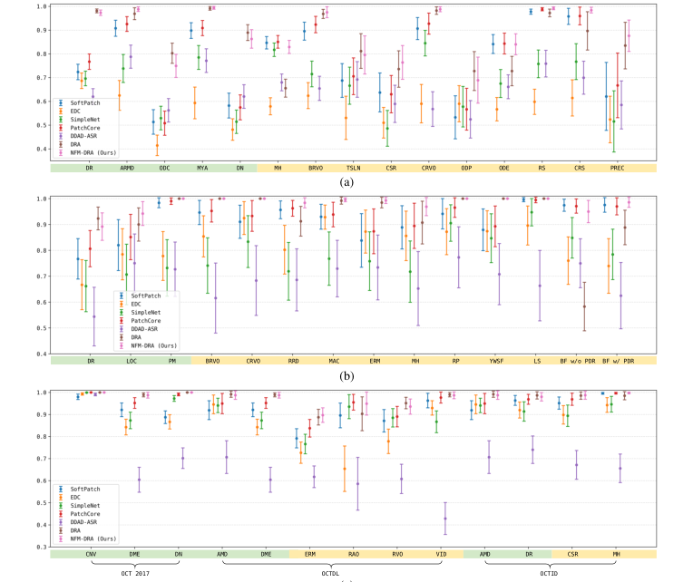Figure 3. AUROCs with 95% confidence intervals for normal samples compared to each abnormal category on the (a) RIADD and (b) JSIEC datasets for fundus benchmarking, as well as (c) OCT test datasets. Seen and unseen annotations highlight whether the anomaly categories appear in the training set or not, respectively

Conversely, PatchCore, a one-class supervised method, exhibited greater robustness to these specific unseen anomalies, often outperforming DRA in those challenging categories. This highlighted a fundamental trade-off: while fully supervised methods can achieve higher peak performance, one-class methods, by focusing solely on learning normal patterns, can sometimes generalize better to truly novel deviations.

This observation directly motivated the development of NFM-DRA. The authors' core mechanism, integrating DRA with a Normal Feature Memory ($M$), was designed to mitigate DRA's robustness issues. The evidence clearly shows this mechanism worked. NFM-DRA achieved the best overall performance, particularly on fundus datasets (RIADD and JSIEC), and maintained comparable performance to DRA on OCT datasets, all while significantly enhancing robustness. It successfully mitigated the performance drops observed in DRA for unseen anomalies like MH and ODE in RIADD, and BF w/o PDR in JSIEC (Figure 3). The mathematical formulation, where the final anomaly score $f(X; M, \text{DRA})$ is a combination of DRA's score and a score derived from comparing test features to the normal feature memory $g(X; M)$, as shown in:
$$ f (X; M, \text{DRA}) = \frac{1}{2} [g (X; M) + \text{DRA} (X)] $$
where $g(X; M)$ is calculated using:
$$ g (X; M) = \left(1 - \frac{\exp (||x^* - m^*||_2)}{\sum_{m \in N^M(m^*)} \exp (||x^* - m||_2)}\right) ||x^* - m^*||_2 $$
and $x^*, m^* = \arg \max_{x \in X} \arg \min_{m \in M} ||x - m||_2$, directly contributed to this improved generalization. The memory bank mechanism allowed NFM-DRA to leverage the learned distribution of normal features to better identify deviations, even when the specific anomaly type had not been seen during training.

Furthermore, the paper provided compelling evidence that the widely used OCT 2017 dataset is no longer adequate as a standalone benchmark. Several models, including DRA, PatchCore, and SimpleNet, achieved near-perfect AUROCs on this dataset, especially for the CNV category (Figure 3c). This performance saturation proves the need for more challenging and diverse benchmarks like BenchReAD to drive future research. Finally, the analysis of threshold-dependent metrics (F1 scores, specificity, and sensitivity) in Tables 1 and 2 revealed that while NFM-DRA achieved the highest average F1 scores, no single method consistently outperformed others across all categories. This highlights the complex nature of real-world clinical deployment, where a model's ability to perform well at specific operating points is crucial, and often more nuanced than a single AUC value suggests.

Limitations & Future Directions

While BenchReAD and NFM-DRA represent a significant step forward, the paper also implicitly and explicitly points to several limitations and opens up exciting avenues for future research.

Limitations:

1. Dataset Saturation (for existing benchmarks): The paper clearly demonstrates that the OCT 2017 dataset, a previously popular benchmark, has reached performance saturation for several advanced models. This means it can no longer effectively differentiate between high-performing algorithms, limiting its utility for future research. While BenchReAD addresses this by incorporating more diverse and challenging datasets, the broader issue of benchmark evolution remains pertinent.
2. Robustness vs. Overall Performance Trade-off: The core finding that fully supervised DRA excels in overall performance but struggles with unseen anomalies, while one-class supervised PatchCore shows greater robustness in those specific cases, highlights a persistent challenge. NFM-DRA mitigates this, but the fundamental tension between maximizing performance on known anomalies and generalizing to truly novel ones is still a complex problem.
3. Variability in Threshold-Dependent Metrics: The F1 scores, specificity, and sensitivity exhibit significant fluctuations across different datasets and anomaly categories. This suggests that even with NFM-DRA's improved average F1, achieving consistent, clinically reliable performance across all possible anomaly types and operating points remains a hurdle. A model might be excellent for one type of anomaly but poor for another, which is a practical limitation for widespread clinical adoption.
4. Computational Resources: The implementation details mention using a single NVIDIA RTX 3090 GPU. While powerful, this might imply that training and extensive benchmarking of these models can be computationally intensive, potentially posing a barrier for researchers with limited access to high-end hardware.

Future Directions & Discussion Topics:

1. Enhancing Generalization to Truly Novel Anomalies: How can we further develop models that are not just robust to unseen anomalies (those absent from training but within a known distribution) but also to truly novel anomalies (those outside the training distribution entirely)? This could involve exploring meta-learning approaches, few-shot anomaly detection, or generative models that can synthesize diverse abnormal patterns to improve model exposure.
2. Adaptive Supervision and Data Efficiency: Given the varying performance across different supervision levels, how can we design intelligent systems that adaptively leverage available data? This might involve dynamic switching between one-class, semi-supervised, and fully supervised components based on the availability and quality of labeled data, or developing active learning strategies to efficiently acquire labels for the most informative samples.
3. Clinical Utility and Decision-Making Integration: The emphasis on threshold-dependent metrics is crucial. How can evaluation protocols be evolved to directly incorporate clinical decision-making frameworks, such as cost-sensitive learning (e.g., penalizing false negatives more heavily than false positives in certain contexts) or utility-based metrics that reflect patient outcomes? This would bridge the gap between algorithmic performance and real-world impact.
4. Explainability and Trust in Medical AI: As these models become more sophisticated, how can we ensure they provide interpretable insights into why a particular region is flagged as anomalous? Clinicians need to understand the basis of a model's prediction to build trust and integrate AI into their workflow. Future work could focus on developing inherently interpretable architectures or post-hoc explanation methods tailored for retinal imaging.
5. Multi-Modal and Longitudinal Anomaly Detection: BenchReAD focuses on two imaging modalities. How can we integrate information from multiple modalities (e.g., OCT, fundus, patient history, genetic data) to improve anomaly detection? Furthermore, how can models be designed to detect changes over time, identifying new anomalies or progression of existing ones in longitudinal patient data, which is critical for disease monitoring?
6. Addressing Data Imbalance and Bias: While BenchReAD provides a more diverse dataset, real-world clinical data often suffers from severe class imbalance and potential biases related to demographics or acquisition protocols. Future research should investigate robust methods for handling extreme data imbalance and ensuring fairness and generalizability across diverse patient populations.

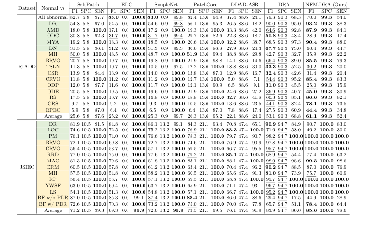Table 1. Threshold-dependent results (%) on fundus test sets, presenting F1 scores, specificity and sensitivity. Categories of seen and unseen anomalies are highlighted to indicate whether they are included in the training set. The best results are shown in bold, and the second-best ones are underlined 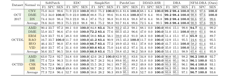Table 2. Threshold-dependent results (%) on OCT test sets, presenting F1 scores, specificity and sensitivity. Seen and unseen anomaly categories are highlighted to show whether they are included in the training set. The best results are in bold and the second-best ones are underlined

Connections to Other Fields

Mathematical Skeleton

The pure mathematical core of NFM-DRA lies in fusing a supervised classification score with a memory-augmented nearest-neighbor-based anomaly score. This latter component quantifies anomaly by assessing the local density of a test feature relative to a stored collection of normal features in a high-dimensional embedding space.

Adjacent Research Areas

Memory-Augmented Anomaly Detection

The proposed Normal Feature Memory (NFM) directly draws inspiration from memory bank mechanisms prevalent in one-class supervised learning for anomaly detection. Specifically, the method computes an anomaly score $g(X; M)$ by finding the closest normal feature $m^*$ in a memory bank $M$ to a representative test feature $x^*$, and then evaluating a similarity metric that incorporates the distance $||x^* - m^*||_2$ and local density information from nearest neighbors in $M$. This approach is a cornerstone of methods like PatchCore, which stores a coreset of normal features to identify deviations, as seen in Roth et al. (2022, IEEE/CVF Conference on Computer Vision and Pattern Recognition).

Open-Set Recognition

The problem NFM-DRA addresses—mitigating performance drops when encountering "unseen anomalies"—is a central challenge in open-set recognition. While the base DRA method is a fully supervised open-set anomaly detector, the NFM component enhances its robustness by providing a direct reference to the distribution of normal samples. This allows the system to identify novel anomalies that were not part of the training set by detecting significant deviations from the learned "normality" stored in the feature memory, a key principle in distinguishing known classes from unknown ones.

Feature Space Density Modeling

The anomaly scoring function $g(X; M)$ implicitly performs a form of local density estimation in the feature space. The term $\frac{\exp(||x^* - m^*||_2)}{\sum_{m \in N^M(m^*)} \exp ||x^* - m||_2}$ can be interpreted as a measure of how "dense" the normal features are around a given test feature $x^*$. A low density of normal features around $x^*$ (i.e., a large distance to $m^*$ or sparse neighbors) contributes to a higher anomaly score. This principle is fundamental to many unsupervised anomaly detection algorithms that model the density of normal data and flag instances in low-density regions as anomalous.