Hybrid Boundary Physics-Informed Neural Networks for Solving Navier-Stokes Equations with Complex Boundary

Background & Academic Lineage

The Origin & Academic Lineage

The problem addressed in this paper originates from the field of computational fluid dynamics (CFD) and the more recent development of Physics-informed Neural Networks (PINNs). Fluid mechanics, which studies the motion of liquids and gases, relies heavily on solving the Navier-Stokes Equations (NSE) – a set of highly nonlinear partial differential equations (PDEs) that describe the dynamic behavior of viscous fluids. Traditionally, CFD methods have been the go-to for these simulations, but they come with inherent challenges, such as the complex and often time-consuming process of mesh generation, potential numerical instability, and sometimes reduced accuracy [2].

In response to these limitations, Physics-informed Neural Networks (PINNs) emerged as a promising alternative. First proposed by Raissi et al. in 2019 [4], PINNs integrate physical prior knowledge (the governing PDEs) directly into a deep learning framework. This innovative approach eliminates the need for mesh generation, a significant advantage over conventional CFD.

However, a fundamental "pain point" quickly became apparent with conventional PINNs, especially when dealing with fluid models involving complex boundary conditions. The core limitation is the "loss conflict problem" [7, 8, 9]. In standard PINN formulations, boundary conditions (BCs) and initial conditions (ICs) are embedded into the neural network's loss function alongside the PDE residual loss. The network is then trained to minimize all these loss components simultaneously. The frequent failure to achieve simultaneous minimization of the PDE residual loss and the boundary condition loss, particularly when boundaries are geometrically intricate, severely compromises the accuracy of the resulting solutions [5]. Even advanced PINN variants designed to mitigate loss balancing issues, like SA-PINN [22] and XPINN [23], still struggle with inaccuracies when faced with highly complex boundary conditions. This persistent challenge of accurately enforcing boundary conditions in complex geometries is the precise problem this paper aims to overcome.

Intuitive Domain Terms

• Physics-informed Neural Networks (PINN): Imagine you're teaching a robot to draw a picture of a car. Instead of just showing it thousands of car pictures (data), you also give it a blueprint of how cars are built and how they move (physics equations). The robot then uses both the visual examples and the engineering rules to draw much more realistic cars, even ones it hasn't seen before. PINNs are like that robot, learning from data while being guided by the fundamental laws of physics.
• Navier-Stokes Equations (NSE): These are essentially the "master rulebook" for how any fluid – like water, air, or even honey – moves. They describe everything from how a river flows to how smoke curls, taking into account factors like speed, pressure, and how "sticky" the fluid is (viscosity). Solving them means accurately predicting the fluid's behavior.
• Complex Boundary Conditions: Think of trying to predict how water flows through a very intricate plumbing system with many twists, turns, narrow pipes, and odd-shaped valves. Simple boundaries would be a straight, smooth pipe. Complex boundaries are all those irregular shapes and specific rules (like "no flow here" or "water enters at this speed") at the edges of the fluid's path. These make the problem much harder to solve accurately.
• Loss Conflict Problem: Picture a juggler trying to keep three balls in the air at once: one representing the physics equations, another the boundary conditions, and the third the initial conditions. If one ball drops (meaning one condition isn't met), the whole act fails. The "loss conflict" is when the juggler finds it incredibly hard to keep all three balls perfectly balanced and in motion, often having to sacrifice the height of one to keep another from falling.
• Distance Metric Network ($N_D$): This is like a specialized "proximity sensor" or "ruler" built into the neural network. For any point within the fluid's domain, this network can instantly tell you how far that point is from the nearest wall or boundary. It's crucial because fluid behavior often changes dramatically as you get closer to a surface, and this network helps the model understand that spatial relationship.

Notation Table

Notation	Description
$N_q(x,t)$	The final composite solution for physical quantity $q$ (e.g., $u, v, p$) at space-time $(x,t)$.
$N_{P_q}(x,t)$	Output of the Particular Solution Network, enforcing boundary conditions for $q$.
$N_{D_q}(x,t)$	Output of the Distance Metric Network, providing boundary-aware weights for $q$.
$N_{H_q}(x,t)$	Output of the Primary Network, solving the governing PDE for $q$.
$L_{PDE}$	Loss component for the PDE residual.
$L_{IC}$	Loss component for initial conditions.
$L_{BC}$	Loss component for boundary conditions.
$\lambda_1, \lambda_2, \lambda_3$	Weighting coefficients for the loss components.
$\hat{D}_q$	True signed distance function for quantity $q$.
$\alpha$	Power-law exponent in the distance metric network.
$u, v$	Velocity components in x and y directions.
$p$	Pressure.
$\rho$	Fluid density.
$\nu$	Dynamic viscosity coefficient.
Re	Reynolds number.
MSE	Mean Squared Error.
MAE	Mean Absolute Error.
L2 error	Relative L2 error.

Problem Definition & Constraints

Core Problem Formulation & The Dilemma

The core problem this paper addresses is the accurate and robust solution of Navier-Stokes Equations (NSE) for fluid dynamics, particularly when dealing with complex boundary conditions. Physics-informed neural networks (PINNs) have shown promise in solving partial differential equations (PDEs), but their application to NSE with intricate geometries remains a significant challenge.

The Input/Current State for this problem is a set of Navier-Stokes Equations, which are highly nonlinear partial differential equations describing viscous fluid motion, along with complex geometric domains and their associated boundary conditions (BCs) and initial conditions (ICs). In conventional PINNs, these BCs and ICs are typically embedded directly into the loss function, alongside the PDE residual loss.

The Desired Endpoint/Goal State is to obtain accurate predictions for physical quantities of interest, such as velocity components ($u, v$) and pressure ($p$), across both the interior domain and at the boundaries, even when these boundaries are geometrically complex. The solution should be robust, stable, and achieve state-of-the-art (SOTA) performance compared to existing PINN-based approaches.

The Exact Missing Link or Mathematical Gap that this paper attempts to bridge lies in the inherent "loss conflict problem" prevalent in conventional PINNs. When boundary conditions are complex, the simultaneous minimization of the PDE residual loss and the boundary condition loss often fails. This is because the network struggles to satisfy both constraints concurrently, leading to compromised accurracy in the resultant solutions. The paper mathematically bridges this gap by proposing a composite solution $N_q(x,t)$ for a physical quantity $q$ (e.g., $u, v, p$) as:

$$ N_q(x,t) = N_{P_q}(x, t) + N_{D_q}(x, t) \cdot N_{H_q}(x, t) $$

Here, $N_{P_q}(x, t)$ is a particular solution network designed to strictly enforce boundary conditions, $N_{D_q}(x, t)$ is a distance metric network that learns boundary-aware weights, and $N_{H_q}(x, t)$ is the primary network focused on resolving the governing PDE. This decoupling, particularly the multiplicative interaction with the distance function, is the novel mathematical mechanism designed to resolve the loss conflict and ensure accurate boundary compliance without sacrificing interior domain accuracy.

The painful trade-off or dilema that has trapped previous researchers is precisely this loss conflict problem: improving the satisfaction of boundary conditions often comes at the expense of accurately solving the governing equations in the interior, and vice-versa. Previous methods, while showing improvements in loss balancing, still suffer from inaccuracies when faced with highly complex boundary conditions. For instance, hard-constrained PINNs (hPINN), which aim to strictly enforce boundary conditions, often exhibit "erratic behavior" and fail to produce reliable results in complex scenarios. Relaxing these strict boundary constraints to improve overall training can lead to solutions that violate fundamental physical requirements, making the compromise unacceptable for scientific modeling.

Constraints & Failure Modes

The problem of solving Navier-Stokes Equations with complex boundary conditions is insanely difficult due to several harsh, realistic constraints:

• Physical/Geometric Complexity: The primary constraint is the intricate geometry of the computational domain. Analytical expressions for particular solutions ($P_q$) and distance functions ($D_q$) are "generally infeasible for complex geometries" (Page 3). This means that traditional methods or simpler PINN architectures struggle to represent the fluid behavior accurately near irregular obstructing structures or segmented inlets, which are common in real-world fluid dynamics.
• Computational/Mathematical Instability:
  • Loss Balancing Challenges: The inherent difficulty in "balancing boundary condition losses and equation losses" (Page 2) leads to "conflicting gradients between equation residuals and boundary condition losses" (Page 5) during neural network training. This makes optimization unstable and prevents simultaneous minimization of all loss components, leading to suboptimal solutions.
  • Overfitting at Boundaries: When boundary condition loss terms are heavily weighted (e.g., $\lambda_2, \lambda_3 \gg \lambda_1$), "excessive training iterations may lead to overfitting in local boundary regions, thereby compromising the global smoothness of the network's output" (Page 24). This means that while the network might perfectly satisfy boundary conditions, its predictions in the immediate interior could be erroneous or non-physical.
  • Differentiability Requirements: Ensuring "global differentiability of the distance function" (Page 3) is a crucial mathematical constraint. Non-differentiable functions would hinder gradient-based optimization methods commonly used in neural networks.
• Empirical Parameter Tuning: Critical parameters, such as the power-law exponent $\alpha$ in the distance metric network and the optimal number of training epochs for the particular solution network ($N_P$), are "currently determined empirically" (Page 10, Limitations; Page 24, C.2; Page 25, C.3). This lack of theoretical guidance for optimal configuration makes the training process highly sensitive and requires extensive trial-and-error, hindering systematic and efficient problem-solving.
• Hardware Memory Limits: While not explicitly detailed as a primary constraint in the problem definition, the paper mentions that the framework is developed on PyTorch and training is "accelerated using a high-performance GPU" (Page 21). This implies that the computational demands of training these deep neural networks for complex fluid dynamics problems are substantial, potentially pushing against hardware memory limits for larger or more complex simulations.

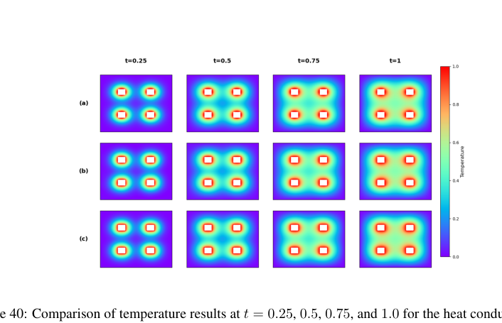Figure 40. Comparison of temperature results at t = 0.25, 0.5, 0.75, and 1.0 for the heat conduction problem: (a) sPINN predictions; (b) HB-PINN predictions; (c) ground truth (GT)

Why This Approach

The Inevitability of the Choice

The development of the Hybrid Boundary Physics-Informed Neural Network (HB-PINN) was not merely an incremental improvement but a necessary architectural shift driven by the inherent limitations of conventional Physics-Informed Neural Networks (PINNs) when confronted with complex boundary conditions. The authors realized that traditional PINN methods, including many state-of-the-art (SOTA) variants, consistently struggled with two critical issues:

First, conventional PINNs embed boundary conditions (BCs) and initial conditions (ICs) directly into the loss function, alongside the partial differential equation (PDE) residual loss. This formulation frequently leads to a "loss conflict problem," where the network fails to simultaneously minimize both the PDE residuals and the boundary condition errors. This issue becomes particularly acute and problematic when the boundary conditions are geometrically intricate or irregular, severely compromising the accuracy of the resulting solutions [7, 8, 9]. The paper explicitly states that "for fluid models with complex boundary conditions, conventional PINN methods often struggle to accurately approximate both the boundary conditions and the partial differential equations [5]." This was the exact moment the authors recognized the insufficiency of existing methods.

Second, while some PINN variants attempted to mitigate this loss conflict, such as those employing distance-informed ansätze [21] or spatially adaptive weighting [22], they still suffered from inaccuracies when dealing with highly complex boundary conditions. Approaches using R-function-based distance functions [25] for boundary enforcement were also found to generate "not natural functions" for complex geometries, indicating a lack of robustness. The core realization was that a fundamental decoupling of the boundary constraint enforcement from the PDE resolution was required to overcome these persistent challenges.

Comparative Superiority

The HB-PINN method achieves qualitative superiority over previous gold standards primarily through its novel, decoupled network architecture and a sophisticated boundary-handling mechanism, rather than solely through simple performance metrics. Its structural advantages are as follows:

1. Decoupled Training Objectives: Unlike conventional PINNs that attempt to minimize PDE and boundary losses simultaneously, HB-PINN employs three specialized subnetworks: $N_P$ (Particular Solution Network), $N_D$ (Distance Metric Network), and $N_H$ (Primary Network). The $N_P$ network is pre-trained to strictly satisfy boundary conditions, and the $N_D$ network learns boundary-condition-aware weights. During the final training phase, only the parameters of $N_H$ are optimized, with $N_P$ and $N_D$ fixed. This design allows $N_H$ to focus exclusively on minimizing the governing PDE residuals, thereby "effectively eliminating the conflicting gradients between equation residuals and boundary condition losses that commonly plague conventional PINN." This is a profound structural advantage that enhances stability and accuracy.

2. Robust Boundary Enforcement: The composite solution $q(x,t) = P_q(x, t) + D_q(x, t) \cdot H_q(x, t)$ (Equation 2) is key. The distance function $D_q$ is designed to be zero at domain boundaries and rapidly increase to one away from them, effectively modulating the influence of the primary network $N_H$ near boundaries. This ensures strict compliance with boundary conditions while allowing $N_H$ to govern the solution in the interior. The introduction of a power-law function $f(D_q) = 1 - (1 - D_q/\max(D_q))^\alpha$ (Equation 9) further refines this distance metric, allowing for tunable steepness near boundaries to accommodate varying complexities. This mechanism provides a more robust and accurate way to handle complex boundaries compared to previous methods that often produced "distorted or discontinuous outputs" near such regions.

3. Enhanced Accuracy in Complex Geometries: The experimental results consistently demonstrate HB-PINN's overwhelming superiority. For instance, across various Reynolds numbers (Table 5), HB-PINN achieves an order-of-magnitude reduction in Mean Squared Error (MSE) compared to conventional methods. This is not just a quantitative win but a qualitative one, as it signifies the method's ability to accurately capture intricate flow dynamics even in regions with high gradients and complex boundary interactions, where other methods fail to produce reliable results (e.g., Figures 3, 6, 9, 30, 32, 34). The ablation studies further confirm that both the particular solution network and the distance metric network are essential for this improved performance, validating the necessity of the composite approach.

Alignment with Constraints

The HB-PINN method is meticulously designed to align with and overcome the harsh requirements of solving Navier-Stokes Equations (NSE) under complex boundary conditions. The "marriage" between the problem's constraints and the solution's unique properties is evident in several aspects:

1. Accurate NSE Solution: The primary network $N_H$ is dedicated to solving the governing PDE. By pre-training and fixing $N_P$ and $N_D$, $N_H$ is freed from the burden of simultaneously satisfying boundary conditions, allowing it to focus solely on minimizing the PDE residual loss (Equation 11). This direct focus ensures a more accurate and stable solution for the NSE in the interior domain.

2. Handling Complex Boundary Conditions: This is the central constraint addressed. The $N_P$ subnetwork is explicitly trained to satisfy boundary conditions, with high loss weighting coefficients ($\lambda_2, \lambda_3 \gg \lambda_1$) to prioritize their enforcement (Equation 5, 6, 4). The $N_D$ subnetwork, parameterized by a DNN, learns a differentiable distance function that smoothly transitions from zero at boundaries to one in the interior. This composite formulation (Equation 3) allows for strict boundary compliance even when analytical expressions for $P_q$ and $D_q$ are infeasible due to complex geometries. This directly tackles the challenge of "irregular obstructing structures" and "segmented inlets" presented in the problem definition.

3. Mitigating Loss Conflict: The core constraint that plagued previous PINNs—the conflict between PDE and BC losses—is directly resolved by HB-PINN's decoupled training strategy. The $N_P$ network handles boundary conditions, and $N_H$ handles the PDE, with $N_D$ mediating their interaction. This prevents the gradients from boundary conditions from interfering with the PDE optimization, leading to more stable and accurate training, especially in scenarios with complex boundaries where this conflict is most pronounced.

4. Mesh-Free Nature: As a PINN-based approach, HB-PINN inherently retains the advantage of eliminating the need for mesh generation, a significant constraint and computational bottleneck in traditional Computational Fluid Dynamics (CFD) methods [2]. This aligns perfectly with the desire for more efficient and flexible surrogate models for fluid dynamics.

Rejection of Alternatives

The paper implicitly and explicitly rejects several alternative approaches, particularly other PINN variants, based on their inability to robustly handle complex boundary conditions and the associated loss conflict problem.

1. Conventional Soft-Constrained PINNs (sPINN): These methods directly add boundary condition losses to the overall loss function. The paper's results (Table 1, Table 5) consistently show sPINN performing significantly worse than HB-PINN, especially in complex scenarios. The implicit rejection is that sPINN's inability to balance PDE and BC losses leads to poor accuracy when boundaries are not simple.

2. Hard-Constrained PINNs (hPINN): While hPINN attempts to enforce boundary conditions strictly, the paper notes its "erratic behavior in scenarios with complex boundary conditions, often failing to produce reliable results" [21]. Appendix D provides a detailed reasoning for its rejection: "for complex boundaries, this approach leads to distorted or discontinuous outputs within the solution domain, especially near junctions between different boundary types." It further explains that hPINN often requires "relaxing the enforcement of boundary conditions in specific subdomains" to achieve effective training, which "violates the requirement for full boundary condition satisfaction" and is "unacceptable for solving physical models." This is a strong, direct rejection of hPINN for the problem at hand.

3. Other Advanced PINN Variants (MFN-PINN, XPINN, SA-PINN, PirateNet): Although these methods offer improvements over basic PINNs, the paper's comprehensive experimental validation (Table 1, Table 5) demonstrates that HB-PINN consistently outperforms them across various complex flow cases and Reynolds numbers. The reasoning for their rejection is that while they "show significant improvements in loss balancing compared to baseline PINN models, they still suffer from inaccuracies when handling problems with highly complex boundary conditions." For instance, MFN-PINN's use of Fourier features might improve approximation capabilities but doesn't fundamentally resolve the boundary condition enforcement issue in the same robust, decoupled manner as HB-PINN. The paper also notes that R-function-based distance functions, used in some variants, are "not natural functions" for complex boundaries.

4. Traditional CFD Methods: The paper's introduction highlights that "challenges such as mesh generation persist and can lead to numerical instability and reduced accuracy" in CFD [2]. PINNs, including HB-PINN, inherently overcome the mesh generation requirement, offering a more efficient and flexible alternative. This constitutes a general rejection of CFD's computational overhead for certain applications. The paper does use CFD results as ground truth, acknowledging its accuracy but emphasizing the advantages of PINNs.

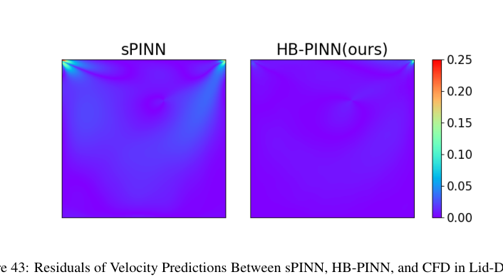Figure 43. Residuals of Velocity Predictions Between sPINN, HB-PINN, and CFD in Lid-Driven Cavity Flow

Mathematical & Logical Mechanism

The Master Equation

The absolute core equation that defines the Hybrid Boundary Physics-Informed Neural Network (HB-PINN) solution for a physical quantity $q$ (such as velocity components $u, v$, or pressure $p$) at a given spatial location $x$ and time $t$ is the composite solution formulation:

$$N_q(x,t) = N_{P_q}(x, t) + N_{D_q} (x, t) \cdot N_{H_q} (x, t)$$

Term-by-Term Autopsy

Let's dissect this equation to understand each component's role and mathematical underpinnings.

• $N_q(x,t)$:

  • Mathematical Definition: This represents the final, predicted value of the physical quantity $q$ (e.g., velocity or pressure) at a specific space-time point $(x, t)$ as output by the entire HB-PINN model. It is a composite function formed by combining the outputs of three distinct neural subnetworks.
  • Physical/Logical Role: This is the ultimate solution that the HB-PINN provides for the partial differential equation (PDE) problem. It aims to accurately represent the physical field (e.g., fluid flow or temperature distribution) across the entire computational domain and over time, while strictly adhering to boundary conditions.
  • Why addition/multiplication: The structure is additive because $N_{P_q}$ provides a baseline solution that satisfies boundary conditions, and $N_{D_q} \cdot N_{H_q}$ represents a "correction" or "refinement" that solves the PDE in the interior. The multiplication within the second term allows $N_{D_q}$ to act as a spatially varying weight, smoothly blending the primary network's contribution.

• $N_{P_q}(x, t)$:

  • Mathematical Definition: This is the output of the Particular Solution Network ($N_P$) for the quantity $q$ at $(x, t)$. $N_P$ is a deep neural network (DNN) with its own set of learnable parameters.
  • Physical/Logical Role: This term's primary role is to enforce strict compliance with the problem's boundary conditions (BCs) and initial conditions (ICs). It acts as a "particular solution" that provides a foundational, boundary-aware component of the overall solution. By pre-training $N_P$ with heavily weighted BC/IC losses, it learns to output values that precisely match the prescribed conditions at the domain edges and initial time.
  • Why it's a separate term: The authors introduced this separate network to decouple the challenging task of satisfying boundary conditions from solving the governing PDE. This strategy mitigates the "loss conflict problem" where gradients from BC losses and PDE losses can interfere, leading to unstable training in conventional Physics-Informed Neural Networks (PINNs).

• $N_{D_q}(x, t)$:

  • Mathematical Definition: This is the output of the Distance Metric Network ($N_D$) for the quantity $q$ at $(x, t)$. $N_D$ is a shallow DNN that is pre-trained to approximate a power-law transformed signed distance function. Specifically, it approximates $f(\hat{D}_q) = 1 - (1 - \hat{D}_q / \max(\hat{D}_q))^\alpha$, where $\hat{D}_q$ is the true signed distance from $(x,t)$ to the nearest boundary. This transformation ensures the output $N_{D_q}(x,t)$ is 0 at the boundaries and approaches 1 as it moves into the domain's interior. The parameter $\alpha$ controls the steepness of this transition.
  • Physical/Logical Role: This term acts as a dynamic, spatially dependent weighting factor for the primary network's output. It serves as a "boundary proximity sensor" or "modulator", ensuring that the influence of the primary network ($N_{H_q}$) is smoothly attenuated to zero at the domain boundaries. This allows $N_{P_q}$ to exclusively dictate the solution at the boundaries, while $N_{H_q}$ contributes fully in the interior.
  • Why multiplication: It multiplies $N_{H_q}$ because it's designed to scale $N_{H_q}$'s contribution. When $N_{D_q}(x,t)$ is zero (at a boundary), it effectively "switches off" $N_{H_q}$'s output, leaving only $N_{P_q}$ to satisfy the boundary condition. As $N_{D_q}(x,t)$ approaches one (in the domain's interior), $N_{H_q}$'s full output is incorporated into the solution.

• $N_{H_q}(x, t)$:

  • Mathematical Definition: This is the output of the Primary Network ($N_H$) for the quantity $q$ at $(x, t)$. $N_H$ is typically a larger DNN compared to $N_P$ and $N_D$.
  • Physical/Logical Role: This term is the main engine for solving the actual governing PDE within the domain. Once $N_P$ and $N_D$ are pre-trianed and fixed, $N_H$ is trained to minimize the PDE residual loss. Its role is to learn the complex, non-linear dynamics of the physical system (e.g., fluid flow, heat transfer) in the interior, free from the burden of strictly enforcing boundary conditions.
  • Why it's a separate term: By offloading boundary condition enforcement to $N_P$ and its smooth integration via $N_D$, $N_H$ can focus entirely on satisfying the physics described by the PDE. This specialized training objective leads to a more stable and accurate learning process, as it avoids the conflicting gradients that arise when a single network tries to simultaneously satisfy both boundary conditions and the PDE.

Step-by-Step Flow

The architecture of our proposed method is illustrated in Fig.1. The framework consists of three subnetworks: $N_P$, $N_D$, and $N_H$. The $N_P$ subnetwork (Particular Solution Network) is trained to satisfy boundary conditions, while the $N_D$ subnetwork (Distance Metric Network) learns boundary-condition-aware weights by encoding the distance from interior points to domain boundaries. The $N_H$ subnetwork (Primary Network) is dedicated to resolving the governing PDE. During the final training phase, only the parameters of $N_H$ are optimized, whereas $N_P$ and $N_D$ remain fixed as pre-trained components. This design effectively addresses challenges involving hybrid interior-exterior boundary configurations. Therefore, we term this methodology Hybrid Boundary Physics-Informed Neural Networks.

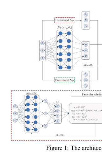Figure 1. The architecture of the proposed method

Imagine a single, abstract data point, representing a specific location and time $(x_i, t_i)$, entering the HB-PINN. Here's how it's processed, like a mechanical assembly line:

1. Input Entry: The space-time coordinate $(x_i, t_i)$ is fed into the HB-PINN architecture. This point could be anywhere in the computational domain, including on or near a boundary.

2. Particular Solution Path: The input $(x_i, t_i)$ first travels to the pre-trained Particular Solution Network ($N_P$). This network, having learned to satisfy boundary conditions, processes the input and outputs a value, $N_{P_q}(x_i, t_i)$. Think of this as a "boundary-compliant blueprint" for the solution at that point.

3. Distance Metric Path: Simultaneously, the same input $(x_i, t_i)$ is sent to the pre-trained Distance Metric Network ($N_D$). This network calculates a value, $N_{D_q}(x_i, t_i)$, which represents how far the point $(x_i, t_i)$ is from the nearest boundary, transformed by a power-law function. This value will be 0 at the boundary and gradually increase to 1 further inside the domain. This is our "boundary influence dial."

4. Primary Solution Path: In parallel, the input $(x_i, t_i)$ also goes into the Primary Network ($N_H$). This network, designed to solve the core physics, computes its raw prediction for the physical quantity at $(x_i, t_i)$, denoted as $N_{H_q}(x_i, t_i)$. This is the "raw physics engine output."

5. Weighted Blending Assembly: The output from the Primary Network, $N_{H_q}(x_i, t_i)$, is then multiplied by the "boundary influence dial" value, $N_{D_q}(x_i, t_i)$. This multiplication step scales $N_{H_q}$'s contribution: if the point is at the boundary ($N_{D_q} = 0$), $N_{H_q}$'s contribution is zeroed out. If the point is deep in the interior ($N_{D_q} \approx 1$), $N_{H_q}$'s full contribution is retained.

6. Final Summation: Finally, the scaled primary solution ($N_{D_q}(x_i, t_i) \cdot N_{H_q}(x_i, t_i)$) is added to the "boundary-compliant blueprint" from the Particular Solution Network, $N_{P_q}(x_i, t_i)$. This sum yields the final composite prediction, $N_q(x_i, t_i)$. This additive step ensures that the boundary conditions are met (primarily by $N_{P_q}$) while the interior solution is accurately informed by the govering PDE (primarily by $N_{H_q}$, modulated by $N_{D_q}$).

Optimization Dynamics

The HB-PINN learns and converges through a carefully orchestrated, multi-stage optimization process that addresses the inherent challenges of balancing different loss components in PINNs.

1. Particular Solution Network ($N_P$) Pre-training:

   • Learning Objective: The $N_P$ subnetwork is initially trained to prioritize the satisfaction of boundary conditions (BCs) and initial conditions (ICs). Its loss function, $L = \lambda_1 L_{PDE} + \lambda_2 L_{IC} + \lambda_3 L_{BC}$ (Equation 4), is heavily weighted towards $L_{IC}$ and $L_{BC}$ (e.g., $\lambda_2, \lambda_3 \gg \lambda_1$).
   • Gradient Behavior & Loss Landscape: This strong weighting creates a loss landscape where gradients from BC and IC errors are dominant. The optimizer (Adam) rapidly drives the network's parameters ($\theta_P$) to configurations that minimize these boundary-related errors. The landscape is shaped to have steep descents towards satisfying the constraints at the domain's periphery and initial time. $N_P$ is trained for a limited number of epochs (e.g., 10,000) to ensure it provides a robust, boundary-compliant baseline without overfitting, which could compromise global smoothness. Once this phase is complete, $\theta_P$ are fixed.

2. Distance Metric Network ($N_D$) Pre-training:

   • Learning Objective: The $N_D$ subnetwork is trained in a supervised manner to approximate a power-law transformed signed distance function. Its loss function, $L_{D_q} = \frac{1}{N_{D_q}} \sum_{i=1}^{N_{D_q}} ||D_q - f(\hat{D}_q)||^2$ (Equation 10), minimizes the squared difference between its output $D_q$ and pre-computed labels $f(\hat{D}_q)$ (where $\hat{D}_q$ is the true signed distance).
   • Gradient Behavior & Loss Landscape: This is a standard regression problem. Gradients guide the network's parameters ($\theta_D$) to accurately map space-time coordinates to the desired distance values (0 at boundaries, 1 in the interior). The parameter $\alpha$ in the power-law function $f(\cdot)$ is crucial here; it shapes the steepness of the transition. An optimal $\alpha$ ensures a smooth yet effective modulatting effect. $N_D$ is trained for a significant number of epochs (e.g., 300,000) to ensure high fidelity in its distance approximation. After training, $\theta_D$ are also fixed.

3. Primary Network ($N_H$) Training:

   • Learning Objective: With $N_P$ and $N_D$ fixed, the $N_H$ subnetwork is trained to minimize the residual of the governing PDE. Its loss function, $L_H = \frac{1}{N_{PDE}} \sum_{i=1}^{N_{PDE}} ||\frac{\partial \hat{u}}{\partial t} + (\hat{u} \cdot \nabla) \hat{u} + \frac{1}{\rho}\nabla \hat{p} - \nu \nabla^2 \hat{u}||^2$ (Equation 11), focuses solely on satisfying the physics equations. The velocity $\hat{u}$ and pressure $\hat{p}$ terms in this loss are derived from the composite solution $N_q(x,t)$ (Equation 3), where $N_P$ and $N_D$ are now static components.
   • Gradient Behavior & Loss Landscape: In this final stage, the gradients exclusively stem from the PDE residual. Critically, because $N_P$ handles boundary conditions and $N_D$ ensures $N_H$'s contribution vanishes at the boundaries, $N_H$ is unburdened by boundary constraints. This results in a much smoother and less conflicting loss landscape for $N_H$, allowing the optimizer to efficiently find parameters ($\theta_H$) that accurately solve the PDE in the domain's interior. Automatic differentiation is used to compute the necessary derivatives for the PDE terms.
   • Convergence: $N_H$ is trained for a large number of epochs (e.g., 300,000-500,000). The Adam optimizer iteratively updates $\theta_H$ to drive the PDE residual towards zero. This focused optimization leads to a robust convergence, yielding a final solution $N_q(x,t)$ that accurately satisfies both the complex boundary conditions and the underlying physical laws. The iterative updates refine the internal representation of the physical fields until the PDE is satisfied to a high degree of accuracy across the domain.

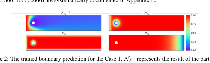Figure 2. The trained boundary prediction for the Case 1. NPu represents the result of the particular solution network for u, while NDu, NDv, and NDp respectively represent the results of the distance metric network for u, v, and p

Results, Limitations & Conclusion

Experimental Design & Baselines

To rigorously validate the Hybrid Boundary Physics-Informed Neural Network (HB-PINN) and definitively prove its efficacy, the authors meticulously designed a series of experiments across diverse fluid dynamics scenarios. The core strategy involved benchmarking HB-PINN against a suite of established Physics-Informed Neural Network (PINN) variants, using high-fidelity Computational Fluid Dynamics (CFD) simulations as the ground truth.

The "victims" (baseline models) chosen for comparison represent a broad spectrum of existing PINN methodologies, including:
* Conventional soft-constrained PINN (sPINN) [4]: The foundational PINN approach where boundary conditions are incorporated into the loss function as soft constraints.
* Hard-constrained PINN (hPINN) [21]: Methods that attempt to strictly enforce boundary conditions, often through architectural design or specific ansatz functions. Notably, the authors found that hPINN exhibited "erratic behavior" and "failing to produce reliable results" in scenarios with complex boundary conditions. To ensure comparability, they selectively relaxed boundary condition enforcement in specific subdomains for hPINN in complex cases, a crucial detail that underscores the challenge HB-PINN aims to overcome.
* Modified Fourier Network PINN (MFN-PINN) [18, 24]: PINNs that leverage Fourier features to better capture high-frequency information.
* Extended PINN (XPINN) [23]: Approaches that use domain decomposition to handle complex geometries.
* Self-adaptive PINN (SA-PINN) [22]: PINNs that dynamically adjust loss weights to mitigate gradient conflicts.
* PirateNets [26]: A recent PINN variant employing residual adaptive networks.

The experimental architecture was designed around three primary two-dimensional incompressible flow cases, each presenting unique challenges:
1. Case 1: Steady-state flow around a circular cylinder (Reynolds number Re = 100). This is a canonical benchmark for fluid mechanics, testing the model's ability to capture wake phenomena.
2. Case 2: Steady-state flow in a segmented inlet with an obstructed square cavity (Re = 100). This case introduces complex inflow boundary conditions and internal obstructions, directly challenging PINNs' ability to handle intricate geometries.
3. Case 3: Transient flow in a segmented inlet with an obstructed square cavity. This extends Case 2 by adding a time-dependent component, further increasing the complexity of boundary and initial conditions.

For all cases, the ground truth (GT) was generated using the Finite Element Method (FEM), ensuring high solution accuracy and numerical stability through dense meshing and a small time step of $\Delta t = 0.01$ for transient simulations.

Beyond these core cases, the authors conducted extensive ablation studies and extended analyses to dissect HB-PINN's components and evaluate its robustness:
* Ablation Studies (Appendix C): These studies ruthlessly isolated the contributions of HB-PINN's two main constructive functions: the particular solution network ($N_P$) and the distance metric network ($N_D$). They compared configurations using only $N_P$ (mP) or only $N_D$ (mD) against the full HB-PINN, demonstrating the necessity of their synergistic combination. Further, they investigated the impact of varying pre-training epochs for $N_P$ and the sensitivity of the power-law exponent $\alpha$ in $N_D$.
* Higher Reynolds Numbers (Appendix G): Case 2 was re-evaluated at elevated Reynolds numbers (Re = 500, 1000, 2000) to test HB-PINN's performance under more turbulent-like conditions.
* More Complex Obstructed Cavity Flow (Appendix H): An even more intricate geometric configuration with staggered obstructions was introduced to push the limits of HB-PINN's ability to handle geometric complexity.
* Other PDE Systems (Appendix I, J): To demonstrate generalizability, HB-PINN was applied to a two-dimensional transient heat conduction problem and a Lid-driven Cavity (LDC) flow, showcasing its potential beyond Navier-Stokes equations.

The entire framework was developed on PyTorch, utilizing high-performance GPUs for accelerated training. Detailed network architectures (number of layers, neurons), activation functions (tanh), optimizers (Adam), learning rates, and specific $\alpha$ values for each subnetwork and case are meticulously documented in Appendix B, ensuring reproducibility.

What the Evidence Proves

The comprehensive experimental validation provides undeniable evidence that HB-PINN significantly outperforms existing PINN-based approaches, particularly in scenarios involving complex boundary conditions. The core mechanism, which decouples boundary condition enforcement into a pre-trained particular solution network ($N_P$) and a boundary-aware distance metric network ($N_D$), while delegating PDE resolution to a primary network ($N_H$), proves to be highly effective.

The definitive evidence can be summarized as follows:

• Superior Accuracy Across Benchmark Cases: Table 1, which quantitatively compares error metrics (Mean Squared Error (MSE), Mean Absolute Error (MAE), and Relative L2 error) across all three main cases, consistently shows HB-PINN achieving the lowest values.
  • For Case 1 (2D cylinder wake flow), HB-PINN's MSE of 0.00433 is remarkably lower than the next best, PirateNet (0.00763), and orders of magnitude better than sPINN (0.52078) or hPINN (0.58347). Figures 3 and 4 visually corroborate this, showing HB-PINN's velocity distributions and residuals to be much closer to the CFD ground truth, with smoother transitions and fewer artifacts compared to baselines.
  • In Case 2 (steady-state obstructed cavity flow), HB-PINN's MSE of 0.00088 is again the lowest, demonstrating a "reduction of an order of magnitude relative to CFD benchmarks" compared to existing methods. The velocity distributions for case 2 from SPINN, hPINN, MFN-PINN, SA-PINN, XPINN, PirateNet and our HB-PINN are shown in Fig.6. Compared to existing methods, the HB-PINN framework demonstrates superior capability in simulating models with complex inflow boundary conditions, achieving a MSE reduction of an order of magnitude relative to CFD benchmarks. The residuals of these methods compared with CFD results are shown in Fig. 7. More detailed error metrics are summarized in the "Case2" section of Table 1.

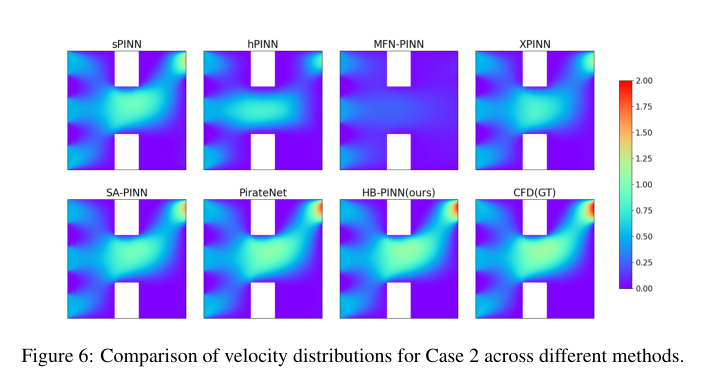Figure 6. Comparison of velocity distributions for Case 2 across different methods

*   For **Case 3 (transient obstructed cavity flow)**, HB-PINN maintains its leading performance with an MSE of 0.00825, outperforming PirateNet (0.03202) and others. Table 4 further breaks down these metrics across multiple time steps ($t=0.1, 0.3, 0.5, 0.7, 1.0$), showing consistent superiority throughout the transient evolution. Figures 9 and 10 illustrate the qualitative accuracy and low residuals. This proves the method's versatility in both steady-state and transient situations.

• Validation of the Hybrid Mechanism through Ablation Studies: The ablation studies (Appendix C, Table 2, Figures 13, 14) are crucial in proving the necessity of HB-PINN's composite architecture.
  • When only the particular solution network (mP) is used, accuracy within the domain is lower.
  • When only the distance metric network (mD) is used, internal errors are reduced, but boundary condition enforcement is imprecise.
  • The fact that the full HB-PINN significantly outperforms both mP and mD configurations (e.g., HB-PINN MSE 0.00088 vs mP 0.00484 and mD 0.00409 for Case 2) provides undeniable evidence that the synergistic combination of these two constructive functions is what enables HB-PINN to sucessfully address the loss conflict problem and ensure accurate solutions in both interior and boundary regions. The comparison of residuals is shown in Fig.8. For a more detailed error analysis, please refer to Table2 in Appendix C.

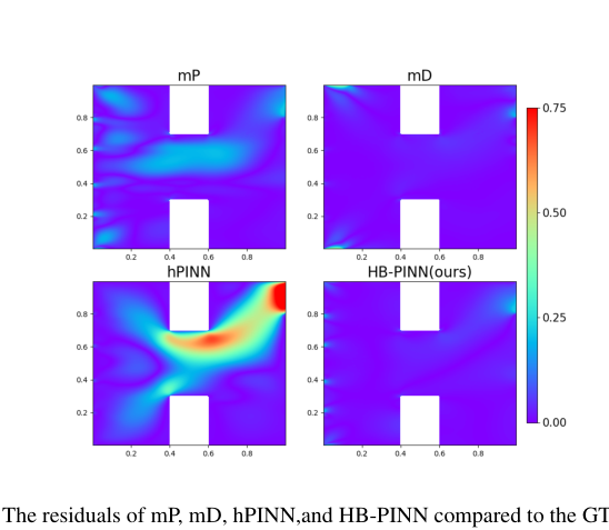Figure 14. The residuals of mP, mD, hPINN,and HB-PINN compared to the GT in Case 2

• Robustness to Increased Complexity and Higher Reynolds Numbers: HB-PINN's performance holds strong even under more challenging conditions.

  • Table 5 and Figure 36 demonstrate that as Reynolds numbers increase (Re = 500, 1000, 2000), all methods show rising prediction errors, but HB-PINN consistently maintains the lowest MSE values. For Re=500, HB-PINN's MSE of 0.00071 represents an order-of-magnitude reduction compared to conventional methods. This highlights the method's robustness and generalizability to more complex flow regimes.
  • In the "more complex obstructed cavity flow" (Appendix H), HB-PINN again significantly outperforms sPINN (Table 6, MSE 0.01331 vs 0.21589), showing its capability to handle intricate geometric structures.

• Applicability to Other PDE Systems: The results for the heat equation and Lid-driven Cavity (LDC) flow (Table 6) extend the evidence beyond Navier-Stokes. For LDC, HB-PINN achieves an MSE of 0.00002, substantially lower than sPINN's 0.00023, indicating its broader utility for various PDE systems with complex boundary conditions.

• Computational Efficiency: Table 7 shows that HB-PINN's training time (47.8 s) is competitive with or faster than many baselines, and its inference time (0.29 s) is significantly faster than traditional CFD (17 s). This demonstrates that the improved accuracy does not come at an exorbitant computational cost, making it a practical surrogate model.

In essence, the evidence proves that HB-PINN's novel architecture, by decoupling boundary constraints and leveraging a distance metric network, effectively resolves the long-standing "loss conflict problem" in PINNs, leading to unparalleled accuracy and robustness in complex fluid dynamics and other PDE problems.

Limitations & Future Directions

While HB-PINN demonstrates state-of-the-art performance and offers a robust solution for complex boundary problems in fluid dynamics, the paper candidly acknowledges certain limitations that pave the way for future research.

One primary limitation highlighted is the empirical determination of critical paramters within the methodology. Specifically, the optimal value for the power-law exponent $\alpha$ in the distance metric network and the ideal number of training iterations for the particular solution network ($N_P$) are currently identified through trial and error. This empirical approach, while effective for the presented cases, lacks a systematic or theoretical foundation, which could become a bottleneck for broader application or when dealing with entirely new problem domains. The paper explicitly states that "Further research is required to systematically identify their optimal configurations."

Based on these limitations and the broader context of PINN research, several promising future directions emerge:

• Automated Hyperparameter Optimization and Adaptive Strategies: A crucial next step is to move beyond empirical tuning for parameters like $\alpha$ and $N_P$ training epochs. Future work could explore advanced optimization techniques such as Bayesian optimization, evolutionary algorithms, or reinforcement learning to automatically discover optimal parameter settings. Alternatively, developing adaptive strategies where these parameters dynamically adjust during training based on real-time error feedback or gradient information could lead to more robust and user-friendly models.
• Theoretical Foundations for Parameter Selection: Deeper theoretical analysis is needed to understand the relationship between these critical parameters and the underlying physics or geometry of the problem. Can we derive analytical bounds or heuristics for $\alpha$ based on boundary complexity or flow characteristics? Such theoretical insights would transform parameter selection from an art to a science, enhancing the generalizability and reliability of HB-PINN.
• Extension to Three-Dimensional and Dynamic Geometries: The current work focuses on 2D incompressible flows. Extending HB-PINN to 3D scenarios, which are ubiquitous in real-world engineering, presents significant computational and architectural challenges. Furthermore, incorporating dynamic or moving boundaries (e.g., fluid-structure interaction with deformable bodies) would push the method's capabilities further, requiring advancements in handling time-varying domains and boundary conditions.
• Integration with Data-Driven Approaches and Hybrid Models: While PINNs are physics-informed, combining HB-PINN with purely data-driven machine learning models could unlock new levels of performance. For instance, using data-driven components to pre-train parts of the network or to refine predictions in regions with high uncertainty could be beneficial. This could lead to truly hybrid models that leverage the strengths of both physical laws and observational data, particularly in scenarios where the governing equations are incomplete or data is abundant.
• Uncertainty Quantification (UQ): For many real-world engineering applications, simply providing a prediction is not enough; understanding the uncertainty associated with that prediction is vital. Future research could integrate UQ techniques (e.g., Bayesian PINNs, ensemble methods) into HB-PINN to provide reliable confidence intervals for its predictions, making it more trustworthy for critical decision-making.
• Computational Scalability and Efficiency for Large-Scale Problems: Although HB-PINN shows good efficiency, scaling it to very large and complex problems (e.g., turbulent flows, global climate models) will require further optimization. This could involve exploring more efficient neural network architectures, distributed computing paradigms, or novel numerical schemes that reduce the computational burden while maintaining accuracy.
• Application to Broader PDE Systems and Multi-Physics Problems: The demonstrated success on heat equations and LDC flow suggests HB-PINN's potential beyond Navier-Stokes. Future work could explore its application to other complex PDE systems in diverse scientific and engineering fields, including electromagnetism, quantum mechanics, or coupled multi-physics problems where different physical phenomena interact.

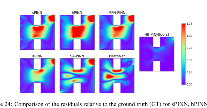Figure 24. Comparison of the residuals relative to the ground truth (GT) for sPINN, hPINN, SA- PINN, XPINN, and our HB-PINN at t = 0.1 in Case 3

Connections to Other Fields

Mathematical Skeleton

The core mathematical contribution involves a constructive decompostion of a PDE solution into a boundary-satisfying component and a residual component, where a learned distance function acts as a smooth blending weight to enforce hard boundary constraints and modulate the influenc of the residual network.

Adjacent Research Areas

Hard-Constrained Physics-Informed Neural Networks

The paper's approach directly builds upon and refines methods for enforcing "hard" boundary conditions in Physics-Informed Neural Networks (PINNs). Specifically, the composite solution $N_q(x,t) = N_{P_q}(x, t) + N_{D_q}(x, t) \cdot N_{H_q}(x, t)$ (Eq. 3) is a learned form of an ansatz, similar to those proposed to analytically satisfy boundary conditions. The function $N_{P_q}$ is designed to satisfy the boundary conditions, while $N_{D_q}$ acts as a "distance-informed" multiplier that is zero at the boundary, ensuring the overall solution $N_q$ adheres to the boundary conditions. This is a direct evolution of techniques like those in Lu et al. (2021, SIAM Journal on Scientific Computing), which use an analytical ansatz to enforce boundary conditions, allowing the main network to focus solely on the PDE residual.

Domain Decomposition Methods for PDEs

The strategy of decoupling the problem into distinct sub-problems—one focusing on boundary conditions ($N_P, N_D$) and another on the interior PDE ($N_H$)—shares conceptual similarites with domain decomposition techniques. While traditional domain decomposition often involves splitting the spatial domain into non-overlapping or overlapping subdomains and solving local PDEs, HB-PINN effectively decomposes the solution space based on proximity to the boundary. The overall solution is a composition of these specialized components, akin to how solutions from different subdomains are stitched together in methods like XPINN (Jagtap and Karniadakis, 2020, Communications in Computational Physics), which uses an interface-informed decomposition framework.

Geometric Modeling and Level Set Methods

The explicit use of a "distance metric network" ($N_D$) to approximate a signed distance function (Eq. 8) is a direct connection to geometric modeling and level set methods. Signed distance functions are fundamental mathematical objects used to implicitly represent complex geometries, where the zero-level set defines the boundary. The power-law function (Eq. 9) applied to this distance function further shapes its behavior near the boundary. This technique is widely used in fields like computer graphics, image processing, and computational geometry for tasks such as shape representation, collision detection, and numerical methods for interfaces, including some PINN variants that use R-functions for distance-based boundary enforcement (Sukumar and Srivastava, 2022, Computer Methods in Applied Mechanics and Engineering).