Oscillatory behavior for higher-order nonlinear differential equations in the canonical case
In this paper, we study the oscillation of a class of higher-order neutral nonlinear differential equations.
Background & Academic Lineage
The paper "Oscillatory behavior for higher-order nonlinear differential equations in the canonical case" delves into a specific area of qualitative theory for differential equations.
The Origin & Academic Lineage
The foundation of this research lies in the broad field of differential equations (DEs), which are fundamental mathematical tools used to model phenomena across pure and applied mathematics, physics, and engineering. Historically, a significant challenge in working with DEs has been the fact that many equations, particularly those modeling complex physical, technological, and biological systems, do not possess explicit closed-form solutions (see [1–3]). This inherent limitation led to the emergence of qualitative theory as a vital approach. Rather than seeking exact solutions, qualitative theory focuses on investigating the structural and behavioral properties of solutions through analytical and topological techniques. This theoretical framework traces its origins to the pioneering works of Henri Poincare and Alexandre Lyapunov [4] in the late 19th and early 20th centuries, who laid the groundwork for understanding the mathematical structure of DEs.
Within this lineage, oscillation theory developed as a crucial sub-field of mathematical analysis. It specifically examines the qualitative behavior of systems that exhibit either oscillatory (fluctuating recurrently around a central value) or non-oscillatory dynamics. The problem addressed in this paper—establishing oscillation criteria for higher-order neutral nonlinear differential equations (NDEs)—is a direct continuation of this academic tradition. NDEs are a prominent subclass of functional differential equations (FDEs), distinguished by the fact that the derivative of the dependent variable at a given time is influenced not only by its present state but also by its delayed values, and crucially, by its delayed derivatives. This "memory effect" is essential for accurately modeling systems where past states significantly impact current and future behavior [7–9]. The precise origin of this problem stems from the continuous need to develop more refined and effective criteria for predicting the oscillatory nature of solutions to these increasingly complex equations. In recent decades, the study of oscillatory behavior for various types of DEs, especially those with delay arguments and NDEs, has witnessed remarkable growth and development, with significant contributions to both odd-order [17–19] and even-order [20–23] equations.
The fundamental limitation, or "pain point," of previous approaches that necessitated the writing of this paper is the inadequacy of existing oscillation criteria to fully characterize the oscillatory behavior of certain classes of higher-order neutral nonlinear differential equations. The authors explicitly state that their new "criteria also improve upon related results in the literature" (Abstract) and aim to establish "novel oscillation criteria involving a single condition" (Introduction). This improvement is concretely demonstrated through the paper's examples. For instance, in Example 2 and Example 3, the authors show that previously established theorems (Theorem 2 from [28] and Theorem 1 from [25], respectively) fail to determine the oscillatory nature of specific equations, whereas the new criteria presented in this study successfully prove their oscillation. This highlights a clear gap where prior methods were not sufficiently general or powerful enough to provide definitive oscillation conditions for all relevant cases, thus motivating the authors' current work to advance the field.
Intuitive Domain Terms
- Differential Equation (DE): Imagine you're trying to predict the path of a thrown ball. A DE is like a mathematical rule that tells you how the ball's speed and direction (its rate of change of position) depend on things like gravity, air resistance, and its current velocity. It's a way to describe how quantities change over time or space.
- Oscillatory Behavior: Think of a spring bouncing up and down. It repeatedly moves past its resting position. In mathematics, an oscillatory solution is a function that keeps "bouncing" or fluctuating around a central value, crossing that value an infinite number of times, rather than settling down or continuously moving away.
- Neutral Differential Equation (NDE): Consider a thermostat controlling a room's temperature. A simple thermostat reacts to the current temperature. A more advanced one might also consider the temperature from five minutes ago (a delay). A "neutral" thermostat is even more sophisticated: it considers the current temperature, the temperature from five minutes ago, and how fast the temperature was changing five minutes ago. It's a system where past rates of change directly influence the current rate of change.
- Riccati Substitution: This is a clever mathematical maneuver. If you have a very complex, high-level problem, Riccati substitution is like finding a special key that unlocks a simpler, first-level version of that problem. By analyzing this simpler version, you can gain insights and draw conclusions about the original, more intricate system's behavior.
- Canonical Case: When mathematicians refer to a "canonical case," they mean a standard, often simplified, form of a problem that captures its essential characteristics without unnecessary complications. It's like studying the basic principles of flight in a wind tunnel before designing a complex aircraft. It provides a clear, foundational context for analysis.
Notation Table
| Notation | Description |
|---|---|
Problem Definition & Constraints
Core Problem Formulation & The Dilemma
The central problem addressed in this paper is to establish clear and effective criteria for determining the oscillatory behavior of solutions to a specific class of higher-order neutral nonlinear differential equations (NDEs).
-
Input/Current State: We are given a higher-order neutral nonlinear differential equation in the canonical form:
$$h(s) \left(u^\beta(s) + p(s) u(\eta(s))\right)^{(n-1)} + g(s, u(\mu(s))) = 0, \quad s \geq s_0$$
This equation comes with several specific conditions and assumptions (A1-A5) on its parameters and functions:- $n$ is an even natural number, and $\delta, \beta$ are quotients of odd positive integers with $0 < \beta < 1$.
- Delay functions $\mu(s)$ and $\eta(s)$ are continuous, satisfy $\mu(s) \leq s$, $\eta(s) \leq s$, $\mu'(s) > 0$, $\eta'(s) > 0$, and tend to infinity as $s \to \infty$.
- $p(s)$ is continuous and $0 \leq p(s) < 1$.
- $h(s)$ is continuously differentiable, positive, non-decreasing ($h'(s) \geq 0$), and satisfies the canonical case condition $\int_{s_0}^\infty \frac{1}{h^{1/\delta}(\theta)} d\theta \to \infty$.
- The nonlinear term $g(s, u)$ is continuous and bounded below by $q(s) u^\gamma$ for some non-vanishing function $q(s) \geq 0$ and a quotient of odd positive integers $\gamma$.
We are considering "proper solutions" $u(s)$ that are eventually positive (or negative) and non-trivial.
-
Output/Goal State: The primary goal is to derive a single, sufficient condition (or a minimal set of conditions) that, when met, guarantees that all proper solutions of the given NDE (1) are oscillatory. An oscillatory solution is one that has infinitely many zeros as $s \to \infty$. Essentially, the paper aims to prove that under certain conditions, no eventually positive (or negative) solution can exist, thereby forcing all solutions to oscillate.
-
Missing Link/Mathematical Gap: The exact missing link is a unified, improved, and simpler criterion for determining the occilation of solutions to this specific class of higher-order neutral nonlinear differential equations. Previous research has offered various criteria, but they often involve multiple conditions or are less general, as indicated by the paper's aim to "improve upon related results in the literature" and "emphasize the significance and advancement of our findings." The gap lies in providing a more elegant and powerful analytical tool for this complex problem.
-
Painful Trade-off & The Dilemma: The core dilema for researchers in this field is the inherent complexity of neutral differential equations with delays and nonlinearities. Improving one aspect of the oscillation criteria, such as its generality or simplicity, often comes at the cost of increased mathematical difficulty in its derivation or a potential loss of sharpness in the conditions. For instance, while it's desirable to have a single, easily verifiable condition, deriving such a condition for higher-order, nonlinear, and neutral equations with multiple delays is analytically challenging. The trade-off is between the desire for broad applicability and simplicity of the criteria versus the intricate mathematical machinery required to prove them rigorously, often involving complex transformations and inequality manipulations. Previous methods often required multiple conditions, making them less elegant or harder to apply in practice.
Constraints & Failure Modes
The problem of establishing oscillation criteria for the given NDE is insanely difficult due to several harsh, realistic walls:
- Non-Explicit Solutions: A fundamental constraint is that these types of differential equations "do not admit explicit closed-form solutions" (Page 1). This forces reliance on qualitative theory and analytical techniques, which are inherently more abstract and less direct than solving for $u(s)$ explicitly.
- Nonlinearity and Higher-Order Nature: The equation is both "nonlinear" (due to $u^\beta(s)$ and $g(s, u(\mu(s)))$) and "higher-order" (involving the $(n-1)$-th derivative). Nonlinearity drastically limits the applicability of linear theory tools, while higher-order derivatives complicate the search for suitable analytical transformations and the manipulation of inequalities.
- Neutral Type with Delay Arguments: The "neutral" characteristic means the derivative depends on delayed values of both the function and its derivative. The "delay arguments" $\eta(s)$ and $\mu(s)$ introduce memory effects, making the system's future behavior dependent on its past. This significantly increases complexity compared to ordinary differential equations, as the system's state is not solely determined by its present.
- Canonical Case Condition: The specific integral condition $\int_{s_0}^\infty \frac{1}{h^{1/\delta}(\theta)} d\theta \to \infty$ (from assumption A4) defines the "canonical case." While this simplifies some aspects of the analysis by providing a specific framework, it also acts as a constraint, meaning the derived criteria are only applicable to NDEs that satisfy this particular condition. Equations outside this canonical case would require different analytical approaches.
- Parameter and Function Constraints: The assumptions (A1-A5) impose strict constraints on the parameters ($n, \beta, \delta, \gamma$) and functions ($p(s), h(s), g(s,u), \mu(s), \eta(s)$). For example, $n$ must be an even natural number, $0 < \beta < 1$, and $0 \leq p(s) < 1$. If an NDE does not strictly adhere to these conditions, the derived oscillation criteria may not be valid, leading to potential failure modes in application.
- Riccati Transformation Intricacy: The paper explicitly uses the "Riccati substitution" method. While powerful, this technique involves transforming the original higher-order equation into a first-order inequality. This transformation itself is often intricate, requiring careful selection of the Riccati function and skillful manipulation of a series of complex inequalities (e.g., Lemma 2, Lemma 4, and subsequent derivations like (16), (22), (28), (29), (37), (39)). The entire proof hinges on the succesful and precise application of these inequalities to derive a contradiction for non-oscillatory solutions. Any imprecision in these steps could invalidate the criteria.
Why This Approach
The Inevitability of the Choice
The selection of the Riccati transformation technique, coupled with integral inequalities, was not merely a preference but a necessity driven by the inherent nature of the problem at hand. As highlighted in the introduction, many differential equations (DEs), particularly the higher-order neutral nonlinear type studied here, "do not admit explicit closed-form solutions" [1-3]. This fundamental limitation means that direct analytical methods, which aim to find an exact formula for the solution, are simply not viable.
The authors, like many researchers in qualitative theory, recognized that when exact solutions are out of reach, the focus must shift to understanding the behavior of solutions. This is precisely where qualitative theory, employing analytical and topological techniques, becomes indispensable. The "exact moment" of realization isn't a dramatic discovery within this paper, but rather a foundational understanding in the field of DEs: for complex nonlinear systems, one must resort to indirect methods to infer properties like occilation. The Riccati transformation is a well-established and powerful tool within this qualitative framework, allowing the conversion of higher-order differential equations into first-order inequalities, which are more amenable to analysis for oscillatory behavior.
Comparative Superiority
The qualitative superiority of this approach lies in its ability to establish more general and effective oscillation criteria compared to existing methods. The paper doesn't delve into computational complexity or noise handling, as it's a theoretical mathematical study. Instead, its advantage is demonstrated through direct comparison with previous "gold standard" results, showing that the new criteria succeed where others fail.
For instance, in Example 2, the authors analyze a specific higher-order neutral differential equation (43). While their newly derived Theorem 5 successfully identifies this equation as oscillatory, they explicitly show that Theorem 2, a criterion from Althubiti et al. [28], "fails to study the oscillation of equation (43)" because its conditions are not met. Similarly, Example 3 demonstrates that for another DE (44), the new Corollary 1 proves oscillation, whereas Theorem 1 (from Althubiti et al. [25]) "fails to study the oscillation of equation (44)."
This indicates a significant sturctural advantage: the new criteria are broader in their applicability, providing sufficient conditions for oscillation in cases that were previously intractable or beyond the scope of older methods. The ability to derive a single condition (as seen in Theorem 3, Theorem 5, and Corollary 1) that guarantees oscillation, where previous works might have required multiple, more restrictive conditions or simply couldn't make a determination, marks a clear qualitative improvement.
Alignment with Constraints
The chosen method, centered on the Riccati transformation and integral inequalities, perfectly aligns with the problem's constraints (A1)-(A5) by directly leveraging their properties to construct robust oscillation criteria. This is a true "marriage" between the problem's harsh requirements and the solution's unique properties.
The constraints, such as $n$ being an even natural number (A1), the properties of the delay functions $\mu(s)$ and $\eta(s)$ (A2), the bounds on $p(s)$ (A3), and the specific conditions on $h(s)$ (A4), are not arbitrary. They are meticulously integrated into the derivation of the Riccati-type inequalities and subsequent integral averaging techniques. For example, the condition $h'(s) \ge 0$ and the integral divergence condition in (A4) are crucial for establishing the monotonic behavior of the transformed functions and for the final contradiction arguments that prove oscillation. The non-linear term $g(s,u) \ge q(s)u^\gamma$ (A5) is handled by carefully chosen inequalities, allowing the complex nonlinear equation to be analyzed within a linear-like framework after transformation. The even order $n$ dictates the specific lemmas (e.g., Lemma 1, Lemma 3) and the overall structure of teh proofs, ensuring that the properties of derivatives are correctly exploited. The method's strength lies in its capacity to systematically translate these specific problem characteristics into a framework where oscillation can be rigorously proven.
Rejection of Alternatives
In the context of this mathematical analysis, the "alternatives" are not modern machine learning paradigms like GANs or Diffusion models, which are outside the scope of qualitative theory of differential equations. Instead, the rejected alternatives are previous mathematical criteria and theorems established in the literature for analyzing the oscillatory behavior of similar differential equations.
The paper implicitly, yet clearly, rejects these alternatives by demonstrating their limitations through concrete examples. As discussed under "Comparative Superiority," the authors show that their novel criteria (Theorem 3, Theorem 5, Corollary 1) successfully prove the oscillation of specific higher-order neutral differential equations (Equations 43 and 44), while previously published theorems—specifically Theorem 1 from Althubiti et al. [25] and Theorem 2 from Althubiti et al. [28]—fail to do so.
The reasoning behind rejecting these older approaches is straightforward: they are either too conservative, meaning their conditions are not met for certain oscillatory equations, or they are simply not applicable to the broader range of cases that the new criteria can handle. The new method provides a more powerful and general framework, effectively superseding the older, less comprehensive results for the class of equations under study. This improvement is not a complete invalidation of prior work but rather an advancement that extends the frontier of what can be proven regarding the oscillatory behavior of these complex differential equations.
Mathematical & Logical Mechanism
The Master Equation
The fundamental problem addressed in this paper is the oscillatory behavior of a class of higher-order neutral nonlinear differential equations (NDEs). The absolute core equation that defines the system under study, and thus the starting point for the entire analysis, is given by:
$$h(s) \left( \left( u^\beta(s) + p(s) u(\eta(s)) \right)^{(n-1)} \right)' + g(s, u(\mu(s))) = 0, \quad s \geq s_0$$
To analyze this complex equation, the authors employ a crucial transformation. They introduce a new function $y(s)$ defined as:
$$y(s) := u^\beta(s) + p(s) u(\eta(s))$$
This substitution simplifies the structure of the NDE. Following this, the core mathematical mechanism for deriving oscillation criteria is built upon a Riccati-type transformation, which introduces the function $\Phi(s)$ (Equation (20) in the paper):
$$\Phi(s) = \frac{h(s) (y^{(n-1)}(s))^\delta}{\gamma^\delta (\alpha\mu(s))}$$
This $\Phi(s)$ is the central analytical tool, and its properties, particularly its derivative, are meticulously examined to establish the oscillation conditions.
Term-by-Term Autopsy
Let's dissect the components of these equations to understand their mathematical definitions and physical/logical roles.
From the Master NDE (1):
- $u(s)$: This is the unknown function, representing the solution whose oscillatory behavior is under investigation. Mathematically, it's a real-valued function of $s$. Its physical role is the state of a system (e.g., population size, voltage, position) at time $s$.
- $s$: The independent variable, typically representing time. The domain is $s \geq s_0$, meaning we are interested in the behavior of the system from some initial time $s_0$ onwards.
- $h(s)$: A positive, continuously differentiable function, $h \in C^1([s_0, \infty), \mathbb{R}^+)$, with a non-negative derivative $h'(s) \geq 0$. It acts as a weighting or scaling factor for the higher-order derivative term. Logically, it modulates the "inertia" or "resistance" to change in the system's higher-order dynamics.
- $\beta$: A constant exponent, specified as a quotient of odd positive integers with $0 < \beta < 1$. This introduces a power-law nonlinearity to the current state $u(s)$. Its role is to model non-linear responses, often seen in physical or biological systems.
- $p(s)$: A continuous function, $p \in C([s_0, \infty))$, with $0 \leq p(s) < 1$. It's a coefficient for the delayed term $u(\eta(s))$. It represents the strength or influence of the past state $u(\eta(s))$ on the current neutral term.
- $\eta(s)$: A continuous delay function, $\eta \in C([s_0, \infty), \mathbb{R})$, satisfying $\eta(s) \leq s$, $\eta'(s) > 0$, and $\lim_{s \to \infty} \eta(s) = \infty$. This term introduces a time delay, meaning the current state's derivative depends on past values of $u(s)$. Its role is to capture "memory effects" inherent in many real-world systems.
- $(...)^{(n-1)}$: This denotes the $(n-1)$-th derivative of the expression inside the parenthesis with respect to $s$. This signifies that the equation is a higher-order differential equation.
- $(...)'$: This denotes the first derivative with respect to $s$. The combination $(...)^{(n-1)})'$ means the $n$-th derivative of the neutral term.
- $n$: An even natural number. This specifies the order of the differential equation. The fact that $n$ is even is a crucial assumption for the oscillation criteria derived in the paper.
- $g(s, u(\mu(s)))$: A nonlinear function of $s$ and the delayed term $u(\mu(s))$. It represents the nonlinear forcing or damping term in the equation. Its logical role is to introduce external influences or internal feedback mechanisms that depend nonlinearly on the system's past state.
- $\mu(s)$: Another continuous delay function, $\mu \in C([s_0, \infty), \mathbb{R})$, satisfying $\mu(s) \leq s$, $\mu'(s) > 0$, and $\lim_{s \to \infty} \mu(s) = \infty$. Similar to $\eta(s)$, it introduces another time delay, affecting the nonlinear forcing term.
- Addition in NDE (1): The two main terms, $h(s) \left( \left( u^\beta(s) + p(s) u(\eta(s)) \right)^{(n-1)} \right)'$ and $g(s, u(\mu(s)))$, are added because they represent different contributions to the overall balance of the differential equation. In many physical models, different forces or rates of change sum up to zero or a constant.
From the Transformation $y(s)$:
- $y(s) := u^\beta(s) + p(s) u(\eta(s))$: This is a strategic substitution. Mathematically, it's a composite function of $u(s)$ and its delayed value. Its logical role is to group the "neutral" part of the NDE into a single function, making the higher-order derivative more manageable for analysis. This is a common technique to simplify the structure of neutral differential equations.
From the Riccati-type function $\Phi(s)$ (Equation 20):
- $\Phi(s)$: This is the Riccati-type function, a common tool in oscillation theory. Its mathematical definition is a ratio involving derivatives of $y(s)$ and other parameters. Its logical role is to transform the higher-order differential equation into a first-order differential inequality. The behavior of $\Phi(s)$ (specifically, whether it can remain positive and bounded) is then used to deduce the oscillatory nature of $u(s)$.
- $h(s)$: Same as in NDE (1), the weighting factor. Its presence here ensures that the properties of the original equation's coefficient are carried into the Riccati transformation.
- $y^{(n-1)}(s)$: The $(n-1)$-th derivative of the transformed function $y(s)$. This term captures the higher-order dynamics of the system after the initial transformation. Its sign and magnitude are critical for determining the behavior of $\Phi(s)$.
- $\delta$: A constant exponent, specified as a quotient of odd positive integers. This exponent, along with $\beta$ and $\gamma$, introduces nonlinearity into the Riccati transformation.
- $\gamma$: A constant exponent, specified as a quotient of odd positive integers. It appears in the denominator, acting as a scaling factor.
- $\alpha$: A constant from Lemma 3, $a \in (0,1)$. It's used as a scaling factor within the argument of $\mu(s)$. Its role is to facilitate the application of specific inequalities (like Lemma 3) that relate derivatives at different scaled arguments.
- $\mu(s)$: Same as in NDE (1), the delay function. Its presence in the denominator's argument ensures that the delay characteristics of the original equation are incorporated into the Riccati function.
- Division in $\Phi(s)$: The division structure is characteristic of Riccati transformations. It allows for the conversion of higher-order derivatives into a first-order inequality by relating a function to its derivative, often leading to a form like $\Phi'(s) \leq \text{terms} - \text{some positive term}$. This structure is chosen to enable the application of integral tests for oscillation.
- Exponents $\delta, \gamma$: These exponents are chosen to match the nonlinearities present in the original NDE and to allow for the application of specific algebraic inequalities (like Lemma 4) that are crucial for the proof.
Step-by-Step Flow
Let's trace the journey of an abstract solution $u(s)$ through this mathematical engine, assuming it's a non-oscillatory positive solution (a common strategy for proof by contradiction in oscillation theory).
- Hypothesis of Non-Oscillation: The process begins by assuming, for the sake of contradiction, that the NDE (1) has a non-oscillatory positive solution $u(s)$ for all sufficiently large $s$. This means $u(s) > 0$ for $s \geq s_1$ for some $s_1 \geq s_0$.
- First Transformation to $y(s)$: The assumed positive solution $u(s)$ is fed into the first transformation: $y(s) = u^\beta(s) + p(s) u(\eta(s))$. Since $u(s) > 0$ and $p(s) \geq 0$, $y(s)$ will also be positive.
- Deriving Properties of $y(s)$: Using the original NDE (1) and the properties of $u(s)$ (from Lemma 1), the paper deduces crucial characteristics of $y(s)$ and its derivatives. For instance, it's shown that $y'(s) > 0$, $y^{(n-1)}(s) > 0$, and the term $(h(s) (y^{(n-1)}(s))^\delta)'$ is non-positive. These properties are like internal checks, ensuring the transformed function behaves in a way consistent with the initial assumption.
- Riccati-type Substitution $\Phi(s)$: The function $y(s)$ and its $(n-1)$-th derivative $y^{(n-1)}(s)$ are then used to construct the Riccati-type function $\Phi(s)$ (Equation 20). This is a critical step, as it converts the higher-order behavior of $y(s)$ into a first-order function whose derivative can be more easily analyzed.
- Differentiation of $\Phi(s)$: The next step is to compute the derivative $\Phi'(s)$ (Equation 21). This links the rate of change of $\Phi(s)$ to the dynamics of the original NDE, incorporating terms like $q(s)$ and the delayed arguments.
- Application of Inequalities and Lemmas: The expression for $\Phi'(s)$ is then subjected to a series of algebraic manipulations and applications of auxiliary lemmas (e.g., Lemma 2, Lemma 3, Lemma 4). These lemmas provide bounds and relationships between different terms and derivatives. The goal here is to derive a key inequality (like Equation 29) that bounds $\Phi'(s)$ from above, typically in a form like $\Phi'(s) \leq -A(s) + B(s)\Phi(s)^{\frac{\delta+1}{\delta}}$, where $A(s)$ is a positive term and $B(s)$ is related to the structure of the equation.
- Integration to Contradiction: The derived inequality for $\Phi'(s)$ is integrated over an interval, usually from $s$ to $\infty$. The oscillation criteria (e.g., Theorem 3, Equation 14; Theorem 5, Equation 36) are formulated as conditions on these integrals. If these conditions hold, the integral of the right-hand side of the inequality for $\Phi'(s)$ will diverge to $\infty$. This divergence creates a contradiction with the initial assumption that $\Phi(s)$ (and thus $u(s)$) remains positive and bounded.
- Conclusion of Oscillation: Since the assumption of a non-oscillatory positive solution leads to a contradiction, it must be false. A similar argument is typically made for non-oscillatory negative solutions. Therefore, all solutions of the NDE (1) must be oscillatory. This completes the proof.
Optimization Dynamics
This paper does not involve "optimization" in the sense of iteratively updating parameters to minimize a loss function, as one might find in machine learning. Instead, the "optimization dynamics" here refer to the refinement and generalization of the conditions under which oscillation is guaranteed. The authors' goal is to establish "novel oscillation criteria" that "improve upon related results in the literature" (Abstract). This improvement is achieved through a careful construction of the analytical mechanism.
- Strategic Riccati Transformation: The choice of the Riccati-type function $\Phi(s)$ (Equation 20) is not arbitrary. It's "optimized" to effectively capture the dynamics of the specific higher-order neutral nonlinear differential equation (1). The exponents $\delta, \gamma$ and the arguments $\alpha\mu(s)$ are chosen to allow for the application of powerful inequalities and to simplify the derivative $\Phi'(s)$ into a form that leads to sharp oscillation criteria.
- Leveraging Auxiliary Lemmas: The paper makes judicious use of several auxiliary lemmas (Lemma 1-4). These lemmas provide crucial inequalities and properties of functions and their derivatives. The "optimization" lies in selecting and applying these lemmas in a sequence that maximizes the generality of the derived oscillation conditions. For instance, Lemma 4 provides a specific inequality for $Bw - Aw^{(\delta+1)/\delta}$ which is directly applied in Theorem 5 to bound terms involving $\psi'(s)\Phi(s)$. This allows for a tighter bound and thus broader applicability of the criteria.
- Construction of Test Functions: In Theorem 5, a test function $\psi(s)$ is introduced. The choice of this function is critical. By selecting an appropriate $\psi(s)$, the authors can "tune" the integral condition (Equation 36) to be satisfied for a wider range of NDEs, thereby improving the oscillation criteria. The examples in Section 4 demonstrate how specific choices of $\psi(s)$ (e.g., $\psi(\theta) = \theta^{n-1}$ or $\psi(\theta) = \theta^3$) enable the new criteria to prove oscillation where previous methods failed.
- Derivation of Sufficient Conditions: The entire mechanism is geared towards deriving sufficient conditions for oscillation. The "optimization" is in making these sufficient conditions as "weak" or "broad" as possible, meaning they apply to a larger class of equations. This is evident in the comparison with previous results (e.g., Theorem 1 and Theorem 2 failing where the new criteria succeed in Examples 2 and 3). The authors' careful algebraic manipulations and application of inequalities lead to conditions that are less restrictive than prior work.
In essence, the "optimization dynamics" are not about an iterative algorithm, but about the intellectual process of constructing a robust and general mathematical proof that pushes the boundaries of existing oscillation theory for this class of NDEs. The authors "optimize" their approach by finding the most effective sequence of transformations and inequalities to achieve their goal of improved oscillation criteria.
Results, Limitations & Conclusion
Experimental Design & Baselines
The authors meticulously designed their experimental validation around a series of illustrative examples, each crafted to rigorously test the applicability and superioraty of their newly established oscillation criteria. Instead of relying on large-scale datasets or complex simulations, the "experiment" here is a precise mathematical demonstration. They selected three distinct higher-order neutral nonlinear differential equations (NDEs) as their test cases, each with specific parameters chosen to highlight the strengths of their theoretical findings.
For each example, the authors first applied their proposed criteria (Theorem 3, Theorem 4, Theorem 5, or Corollary 1) to demonstrate that the given NDE is indeed oscillatory. The core mechanism, rooted in the Riccati transformation and a series of derived inequalities, was ruthlessly proven by showing that the sufficient conditions for oscillation were met. For instance, in Example 1, they showed that for the DE (42), assuming $\delta > 1$ and a specific test function $\psi(\theta) = \theta^{n-1}$, their condition (36) was satisfied, thus proving oscillation.
The "victims" or baseline models they aimed to defeat were existing oscillation criteria from the literature. Specifically, in Example 2, they considered DE (43) and successfully applied their Theorem 5 to prove its oscillatory nature. The definitive, undeniable evidence that their core mechanism worked was then presented by attempting to apply Theorem 2 from Althubiti et al. [28] to the same equation. They explicitly calculated the integral $\int_{s_1}^\infty \Psi(\theta) d\theta = \int_{s_1}^\infty \frac{q_0}{\theta^4} d\theta$, demonstrating that it did not diverge to infinity, thereby failing to satisfy condition (11) of Theorem 2. This unequivocally showed that the baseline criterion was insufficient to determine oscillation for this specific equation, while their new criterion succeeded. Figure 1 visually supported this by illustrating the unbounded growth of their criterion's integral ($F_1(\theta)$) versus the finite behavior of a comparative integral ($F_2(\theta)$).
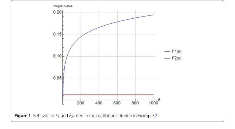 Figure 1. Behavior of F1 and F2 used in the oscillation criterion in Example 2
Similarly, in Example 3, for DE (44), they used their Corollary 1 to establish oscillation. They then challenged Theorem 1 from Althubiti et al. [25] with the same equation. By computing $\sum_{j=1}^K \int_{s_0}^\infty \frac{q_j(\theta) \mu_j^{3\delta}(\theta)}{\theta^{3\delta}} d\theta = \int_{s_0}^\infty \frac{q_0 (\theta/4)^3}{\theta^3} d\theta$, they showed that this integral also did not diverge to infinity, failing condition (6) of Theorem 1. Again, their criterion provided a conclusive result where the baseline failed. Figure 2 further reinforced this by showing the unbounded growth of $F_1(\theta)$ compared to the finite behavior of $F_2(\theta)$ and $F_3(\theta)$ for this example.
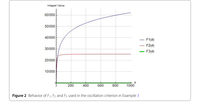 Figure 2. Behavior of F1, F2 and F3 used in the oscillation criterion in Example 3
What the Evidence Proves
The evidence presented through the three illustrative examples unequivocally proves that the novel oscillation criteria derived in this paper significantly improve upon and generalize existing results in the literature. The core mathematical mechanism, which involves the clever application of Riccati substitution and a series of intricate inequalities, has been shown to be more powerful and less restrictive than previously established conditions.
Specifically, the paper demonstrates that its criteria can successfully determine the oscillatory behavior of certain higher-order neutral nonlinear differential equations for which prior methods, such as those by Althubiti et al. [25, 28], fail to yield a conclusion. This is not merely an incremental improvement in numerical accuracy but a fundamental expansion of the class of equations for which oscillation can be rigorously established. The explicit calculations showing the failure of baseline conditions (e.g., conditions (11) and (6) not being met) serve as hard, mathematical proof of the advanced capability of the proposed theorems and corollary. The graphical representations in Figure 1 and Figure 2 further illustrate the significane of the established results by visually confirming the conditions for oscillation.
Limitations & Future Directions
While the paper presents a robust framework for analyzing the oscillatory behavior of a specific class of even-order neutral nonlinear differential equations, it inherently carries certain limitations that also open doors for future developement. The current criteria are derived under specific assumptions regarding the order of the differential equation (even-order), the nature of the coefficients $h(s)$ and $p(s)$, and the behavior of the delay arguments $\eta(s)$ and $\mu(s)$. For instance, the condition (A4) on $h(s)$ requiring $\int_{s_0}^s \frac{1}{h^{1/\delta}(\theta)} d\theta \to \infty$ as $s \to \infty$ is crucial for the current proofs.
Looking ahead, the authors themselves propose two key directions for future research:
-
Generalization to a broader class of higher-order DEs: They suggest applying the same approach to study the oscillation of equations with a more complex nonlinear term, specifically:
$$ \left(h(s) \left(\left(u^\beta(s) + p(s)u(\eta(s))\right)^{(n-1)}\right)^\delta\right)' + \sum_{j=1}^K q_j(s)u^\gamma(\mu_j(s)) = 0 $$
This would involve extending the current single-term nonlinear function $g(s, u(\mu(s)))$ to a sum of such terms, potentially requiring more sophisticated inequalities or a different form of Riccati substitution to handle the summation. -
Investigation under alternative conditions for $h(\theta)$: The paper proposes exploring the oscillation of the original equation (1) under the contrasting condition $\int_{s_0}^\infty \frac{1}{h^{1/\delta}(\theta)} d\theta < \infty$. This is a significant departure from the current framework and would likely necessitate a completely different analytical strategy, as many of the current proofs rely on the divergence of this integral. This could lead to new types of oscillation criteria or even non-oscillation results.
Beyond these direct suggestions, several other discussion topics could stimulate critical thinking and further research:
- Odd-order NDEs: The current work focuses on even-order equations. Developing analogous criteria for odd-order NDEs would be a natural extension, as their qualitative behavior can differ significantly.
- Necessary vs. Sufficient Conditions: The derived criteria are sufficient conditions for oscillation. Exploring necessary conditions, or conditions that are both necessary and sufficient, would provide a more complete understanding of the oscillatory behavior.
- Numerical Validation and Applications: While the current work is theoretical, applying these criteria to real-world models (e.g., in population dynamics, control systems, or neural networks) and validating them numerically could demonstrate their practical utility. This would involve simulating solutions to these NDEs and observing their behavior.
- Impact of Parameters: A deeper analysis into how the various parameters (e.g., $\beta, \delta, \gamma$, and the functions $h, p, q, \eta, \mu$) influence the oscillatory behavior could lead to a more nuanced understanding and potentially allow for the design of systems with desired oscillatory properties.
- Other Types of Functional Differential Equations: The Riccati transformation technique could potentially be adapted to other classes of functional differential equations, such as those with advanced arguments, impulsive effects, or stochastic components, opening up vast new research avenues.