Flow Straight and Fast: Learning to Generate and Transfer Data with Rectified Flow
Rectified Flow learns straight paths to efficiently generate and transfer data between distributions.
Background & Academic Lineage
The Origin & Academic Lineage
The problem of transporting one probability distribution to another—often called the "transport mapping problem"—is a foundational challenge in machine learning and statistics. Historically, this problem emerged from the field of Optimal Transport (OT), which seeks to find the most efficient way to move mass between distributions. While OT provides a rigorous mathematical framework, it is notoriously difficult to solve in high-dimensional spaces, such as those encountered in modern image generation or domain transfer tasks.
Previous approaches, particularly generative models like Generative Adversarial Networks (GANs) and Variational Autoencoders (VAEs), attempted to solve this by learning mappings between data and latent spaces. However, these models often suffer from significant pain points: GANs are plagued by numerical instability and mode collapse, while VAEs and other likelihood-based models often require complex, computationally expensive inference procedures. More recently, continuous-time models like diffusion models and neural Ordinary Differential Equations (ODEs) have gained popularity. While powerful, these models are essentially "infinite-step" processes; they require solving complex differential equations by repeatedly calling an expensive neural network, which makes real-time application or fast inference prohibitively slow. The authors of this paper identified that the core limitation of these continuous-time models is their reliance on curved, non-straight trajectories, which necessitate many discretization steps to simulate accurately.
Intuitive Domain Terms
- Rectified Flow: Think of this as "straightening the highway." Instead of letting data particles travel along winding, inefficient paths between two distributions, this method forces them to follow the shortest possible straight-line path, making the journey much faster and easier to calculate.
- Reflow: Imagine a delivery driver who takes a winding route on their first day. After observing the traffic, they "reflow" their route to be a perfectly straight line. By iteratively training on the paths generated by the previous model, the system "straightens" its own trajectories, allowing for high-quality results with far fewer steps.
- Coupling: This is simply a "pairing plan." If you have a pile of sand (distribution $\pi_0$) and want to move it into a specific shape (distribution $\pi_1$), a coupling is the set of instructions that tells every individual grain of sand exactly where to go.
- Drift Force: In the context of ODEs, this is the "steering wheel" of the model. It is a neural network that tells the data points which direction to move at any given time $t$ to ensure they arrive at their destination.
- Discretization Step: Think of this as the "frame rate" of a video. To simulate a continuous movement, we break it into small chunks. A high number of steps means a smooth but slow process; the authors aim to achieve high quality with a very low number of steps (even just one).
Notation Table
| Notation | Description |
|---|---|
| $\pi_0, \pi_1$ | The two probability distributions (source and target) being connected. |
| $X_0, X_1$ | Random variables drawn from $\pi_0$ and $\pi_1$, respectively. |
| $Z_t$ | The state of the flow at time $t \in [0, 1]$. |
| $v(Z_t, t)$ | The velocity field (drift) that determines the movement of the flow. |
| $X_t$ | The linear interpolation between $X_0$ and $X_1$, defined as $tX_1 + (1-t)X_0$. |
| $S(\mathbf{Z})$ | A measure of "straightness" for a flow; lower values indicate straighter paths. |
| $N$ | The number of discretization steps used for numerical simulation. |
| $\theta$ | The parameters of the neural network used to approximate the velocity field. |
Problem Definition & Constraints
Core Problem Formulation & The Dilemma
The paper addresses the fundamental problem of learning a transport map between two empirically observed data distributions, $\pi_0$ and $\pi_1$, in high-dimensional spaces. This is a crucial task for various machine learning applications, including generative modeling (e.g., mapping Gaussian noise to images) and domain transfer (e.g., translating images from one style to another).
Input/Current State: The starting point is having empirical observations (samples) from two distributions, $\pi_0$ and $\pi_1$, typically in $\mathbb{R}^d$. A critical aspect of this problem is the lack of paired input/output data. That is, for each sample $X_0 \sim \pi_0$, there isn't a corresponding $X_1 \sim \pi_1$ that is known to be its "correct" translation or generation target. Instead, we only have independent sets of samples from each distribution.
Output/Goal State: The desired endpoint is to learn a transport map $T: \mathbb{R}^d \to \mathbb{R}^d$ such that, in the infinite data limit, if $Z_0 \sim \pi_0$, then $Z_1 := T(Z_0) \sim \pi_1$. More specifically, the paper aims to learn a neural ordinary differential equation (ODE) model, $dZ_t = v(Z_t, t)dt$, that can transport samples from $\pi_0$ to $\pi_1$ by following paths that are as "straight" as possible. This ODE should be simulable forwardly to generate new data or perform domain transfer.
Missing Link/Mathematical Gap: The exact missing link is how to construct a causal and computationally efficient transport map from unpaired data that unifies generative modeling and domain transfer, while overcoming the limitations of existing methods.
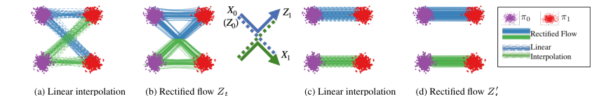 Figure 2. (a) Linear interpolation of data input (X0, X1) ∼π0 × π1. (b) The trained rectified flow Zt ; the trajectories are “rewired” at the intersection points to avoid crossing. (c) The linear interpolation of the end points (Z0, Z1) of flow Zt. (d) The rectified flow induced from (Z0, Z1), which follows straight paths
Previous attempts to bridge this gap faced several issues:
1. Naive Linear Interpolation: A simple linear interpolation $X_t = tX_1 + (1-t)X_0$ provides straight paths but is "non-causal (or anticipating)." It requires knowing the final point $X_1$ to determine $X_t$, making it impossible to simulate forwardly to generate new data.
2. Optimal Transport (OT): While OT provides a theoretically sound framework for finding mappings that minimize transport costs, it is "highly challenging computationally" for high-dimensional continuous measures and often "not of direct interest" for the specific objectives of many machine learning tasks.
3. Continuous-Time Generative Models (ODEs/SDEs): Recent advances in models like score-based generative models and denoising diffusion probabilistic models (DDPM) have shown impressive results. However, these models are "effectively 'infinite-step'" and incur "high computational cost in inference time" because they require repeatedly calling an expensive neural force field for a large number of times to simulate the ODE/SDE.
The paper attempts to bridge this gap by formulating the problem as a straightforward nonlinear least squares optimization. It seeks to learn a velocity field $v(Z_t, t)$ that drives the ODE $dZ_t = v(Z_t, t)dt$ to follow the direction of the linear paths $(X_1 - X_0)$ as closely as possible, where $X_t = tX_1 + (1-t)X_0$ is the linear interpolation between empirically sampled points. This is expressed as:
$$ \min_v \mathbb{E} \left[ \int_0^1 \|(X_1 - X_0) - v(X_t, t)\|^2 dt \right] $$
This formulation aims to "causalize" the straight paths of linear interpolation, making them simulable.
Constraints & Failure Modes
The problem of learning transport maps between distributions is constrained by several harsh, realistic walls:
Physical, Computational, or Data-driven Constraints:
* Unpaired Data: The most significant data-driven constraint is the inherent "lack of paired input/output data" in unsupervised learning settings. This means the model cannot simply learn a direct regression from $X_0$ to $X_1$.
* High-Dimensionality of Data: Real-world data, especially images, exists in very high-dimensional spaces ($\mathbb{R}^d$ where $d$ can be millions). This makes direct optimal transport computations intractable and exacerbates the computational cost of numerical ODE/SDE solvers.
* Computational Cost of ODE/SDE Solvers: Existing continuous-time models require "repeatedly call the expensive neural force field for a large number of times" during inference. This translates to strict real-time latency requirements in many applications, where generating an image in hundreds or thousands of steps is too slow.
* Non-Crossing Property of ODEs: For a well-defined ODE, its solution must be unique, meaning different paths cannot cross each other. This is a fundamental mathematical constraint that any learned flow must satisfy, unlike naive linear interpolations which can intersect.
Why This Approach
The Inevitability of the Choice
The authors identified that traditional generative models—specifically GANs and diffusion models—hit a fundamental "computational wall" regarding inference speed. GANs, while fast, suffer from notorious training instability and mode collapse. Conversely, diffusion models (and their ODE-based variants like PF-ODEs) are mathematically robust but computationally expensive because they require solving complex, curved trajectories that necessitate many discretization steps to maintain accuracy. The authors realized that the "curved" nature of these trajectories was the primary bottleneck; if the transport path between two distributions could be made "straight," the ODE could be solved with minimal discretization, potentially even a single step. This realization shifted the focus from merely matching distributions to finding the shortest, straightest path between them.
Comparative Superiority
Rectified flow is qualitatively superior because it transforms the transport problem into a simple, scalable, unconstrained least squares optimization. Unlike GANs, which require delicate minimax balancing, or diffusion models, which rely on complex SDE/ODE solvers, rectified flow uses a "reflow" procedure. This procedure iteratively straightens the trajectories of the flow. Structurally, this reduces the discretization error significantly. While standard diffusion models might require hundreds of function evaluations (NFE) to produce high-quality images, rectified flow—especially after reflow—can produce comparable or superior results with a single Euler step. This effectively bridges the gap between one-step models (like VAEs) and continuous-time models, offering the high quality of the latter with the speed of the former.
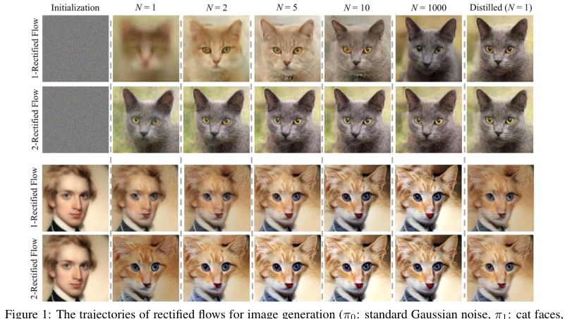 Figure 1. The trajectories of rectified flows for image generation (π0: standard Gaussian noise, π1: cat faces, top two rows), and image transfer between human and cat faces (π0: human faces, π1: cat faces, bottom two rows), when simulated using Euler method with step size 1/N for N steps. The first rectified flow induced from the training data (1-rectified flow) yields good results with a very small number (e.g., ≥2) of steps; the straightened reflow induced from 1-rectified flow (denoted as 2-rectified flow) has nearly straight line trajectories and yield good results even with one discretization step. problem of finding an optimal coupling that minimizes a notion of transport cost, typically of form E[c(Z1 −Z0)], where c: Rd →R is a cost function, such as c(x) = ∥x∥2. However, for the gen- erative and transfer modeling tasks above, the transport cost is not of direct interest, even though it induces a number of desirable properties. Hence, it is not necessary to accurate solve the OT problems given the high difficulty of doing so. An important question is to identify relaxed notions of optimality that are of direct interest for ML tasks and are easier to enforce in practice
Alignment with Constraints
The problem constraints required a model that could handle high-dimensional data (like images) without the instability of GANs or the prohibitive inference cost of diffusion. Rectified flow aligns with these constraints through its "causalization" of the transport path. By training the drift force $v$ to follow the linear interpolation $X_t = tX_1 + (1-t)X_0$, the model learns to transport mass in a myopic, non-crossing, and deterministic way. This "marriage" of the ODE framework with a straight-line objective ensures that the model is both computationally efficient (due to the straight paths) and theoretically sound (as it preserves marginal distributions and reduces transport costs).
Mathematical & Logical Mechanism
The Master Equation
The core mechanism of Rectified Flow is to learn a velocity field $v(z, t)$ that transforms a source distribution $\pi_0$ into a target distribution $\pi_1$ by following straight-line paths. The objective function used to train this velocity field is:
$$\min_{v} \int_{0}^{1} \mathbb{E} \left[ \left\| (X_1 - X_0) - v(X_t, t) \right\|^2 \right] dt, \quad \text{with } X_t = tX_1 + (1 - t)X_0$$
Step-by-Step Flow
- Initialization: A pair $(X_0, X_1)$ is sampled from the data distributions.
- Interpolation: The system calculates the intermediate point $X_t$ at a randomly sampled time $t$.
- Velocity Prediction: The neural network $v$ takes the current state $X_t$ and time $t$ as input and outputs a predicted velocity vector.
- Regression: The model compares its predicted velocity against the target direction $(X_1 - X_0)$.
- Update: The network parameters are updated via gradient descent to minimize the difference.
- Inference: During sampling, the model starts at $Z_0 \sim \pi_0$ and solves the ODE $dZ_t = v(Z_t, t)dt$ using a numerical solver (like Euler's method) to reach $Z_1 \sim \pi_1$.
Optimization Dynamics
The mechanism learns by "causalizing" the linear interpolation. While the naive path $X_t$ requires knowledge of the future ($X_1$), the learned velocity field $v(Z_t, t)$ is a function only of the current state and time, making it a valid, causal ODE.
The "reflow" procedure is a critical optimization dynamic: after training an initial model, the model is used to generate new pairs $(Z_0, Z_1)$ by simulating the learned flow. These new pairs are used to retrain the model. Because the flow generated by the first model is already "straighter" than the raw data coupling, the second iteration produces even straighter paths. This iterative process effectively "straightens" the flow, reducing the discretization error of numerical solvers. Consequently, the loss landscape becomes increasingly smooth, allowing the model to converge to a state where high-quality samples can be generated with very few (or even one) Euler steps.
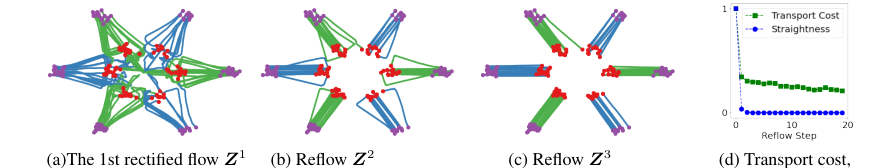 Figure 3. (a)-(c) Trajectories of the reflows on a toy example (π0: purple dots, π1: red dots; the green and blue lines are trajectories connecting different modes of π0, π1). (d) The straightness and the relative L2 transport cost v.s. the reflow steps. See Appendix D.5 for more information
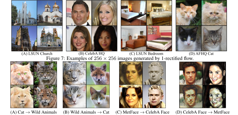 Figure 9. Samples of results of 1- and 2-rectified flow simulated with N = 1 and N = 100 Euler steps. Experiment settings We set the domains π0, π1 to be pairs of the AFHQ (Choi et al., 2020), MetFace (Karras et al., 2020) and CelebA-HQ (Karras et al., 2018) dataset. The results are shown by initializing the trained flows from the test data. The training and network configurations follow Section 3.1. See Appendix E for details
Results, Limitations & Conclusion
Experimental Design & Baselines
The authors evaluate Rectified Flow primarily on unconditional image generation using the CIFAR-10 dataset and high-resolution datasets (LSUN, CelebA-HQ, AFHQ). To establish a rigorous baseline, they utilize the U-Net architecture from the DDPM++ framework (Song et al., 2020b). The experimental design is structured to test the efficacy of the "reflow" procedure and the resulting "straightness" of the learned ODE trajectories.
What the Evidence Proves
The evidence provided is compelling, particularly regarding the "straightening" effect of the reflow procedure. The authors demonstrate that while the initial (1-rectified) flow is effective, it is not perfectly straight. By applying the reflow procedure—where the model is retrained on data generated by the previous flow—the trajectories become increasingly linear.
The definitive evidence for this mechanism is twofold:
* Quantitative: On CIFAR-10, the distilled 2-rectified flow achieves an FID of 4.85, which significantly outperforms the best-known one-step generative model (TDPM, FID 8.91). Furthermore, the recall of 0.51 exceeds that of StyleGAN2+ADA (0.49), proving that the method maintains high diversity.
* Visual/Geometric: Figure 4 and Figure 18 provide visual proof that the trajectories of the 2-rectified flow are nearly straight lines. The extrapolation $\hat{z}_1^t = z_t + (1-t)v(z_t, t)$ remains almost constant regardless of $t$, which is a hallmark of a straight-line ODE. This confirms that the model has successfully "causalized" the transport process, allowing for accurate simulation with minimal discretization steps.
Limitations & Future Directions
Future directions for this research could include:
* Theoretical Refinement: Exploring whether there exists a theoretical limit to the number of reflow steps before the accumulation of numerical error outweighs the benefits of trajectory straightening.
* Broader Applications: Investigating if the "straightening" property can be leveraged in non-generative tasks, such as physical system modeling or time-series forecasting.
* Optimal Transport Integration: As the authors mention, rectified flow does not strictly guarantee $c$-optimal transport for a specific cost function $c$. Future work could focus on constraining the velocity field $v$ to be a gradient field (e.g., $v = \nabla f$) to explicitly enforce optimality.
These findings suggest a paradigm shift in generative modeling: moving away from the "noise-to-data" diffusion paradigm toward a "straight-line" transport paradigm, which is computationally more efficient and theoretically more transparent.
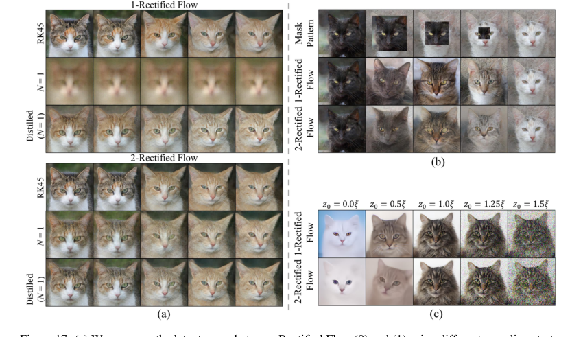 Figure 17. (a) We compare the latent space between Rectified Flow (0) and (1) using different sampling strate- gies with the same random seeds. We observe that (i) both 1-Rectified Flow and 2-Rectified Flow can provide a smooth latent interpolation, and their latent spaces look similar; (ii) when using one-step sampling (N = 1), 2-Rectified Flow can still provide visually recognizable interpolation, while 1-Rectified Flow cannot; (iii) Dis- tilled one-step models can also continuously interpolate between the images, and their latent spaces have little difference with the original flow. (b) We composite the latent codes of two images by replacing the boundary of a black cat with a white cat, then visualize the variation along the trajectory. The black cat turns into a grey cat at first, then a cat with mixing colors, and finally a white cat. (c) We randomly sample ξ ∼N(0, I), then generate images with αξ to examine the influence of α on the generated images. We find α < 1 results in overly smooth images, while α > 1 leads to noisy images
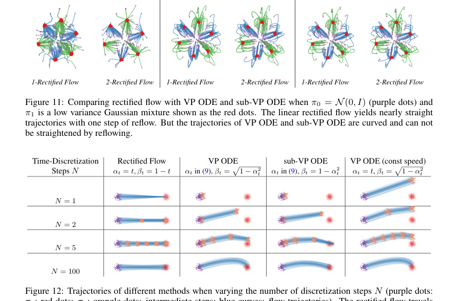 Figure 12. Trajectories of different methods when varying the number of discretization steps N (purple dots: π0; red dots: π1; orangle dots: intermediate steps; blue curves: flow trajectories). The rectified flow travels in straight lines and progresses uniformly in time; it generates the mean of π1 when simulated with a single Euler step, and quickly covers the whole distribution π1 with more steps (in this case N = 2 is sufficient). In comparison, VP ODE and sub-VP ODE travel in curves with non-uniform speed: they tend to be slow in the beginning and speed up in the later phase (much of the update happens when t⪆0.5). The non-uniform speed can be avoided by setting αt = t (see the last column)
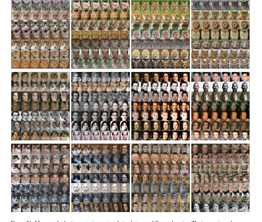 Figure 21. More results for image-to-image translation between different domains. The images in each row are time-uniformly sampled from the trajectory of 1-rectified flow solved N = 100 Euler steps with constant step size