Beyond Shadows: Learning Physics-inspired Ultrasound Confidence Maps from Sparse Annotations
ISOM keeps this paper as an uncertainty-field example: confidence maps become part of inference rather than an after-the-fact diagnostic.
Background & Academic Lineage
The Origin & Academic Lineage
The problem of generating reliable confidence maps in ultrasound imaging is not new; it has been a persistent challenge in medical image analysis for quite some time. Ultrasound itself is a widely used diagnostic tool, valued for its non-invasive nature, real-time capabilities, and cost-efficiency. Confidence maps emerged as a way to quantitatively assess the reliability of each pixel within an ultrasound image, providing crucial information for various downstream applications. Historically, these maps have been employed in areas such as intensity reconstruction, volume compounding, US-CT registration, shadow detection, and deep learning segmentation. More recently, their utility has expanded to robotic ultrasound for tasks like probe positioning and contact force optimization.
However, previous approaches to generating these confidence maps faced significant limitations, which motivated the authors to develop this novel method. A primary "pain point" was that existing physics-based models often overlooked common ultrasound artifacts, such as reverberation, leading to inaccurate confidence assessments. Shadow-based models, while useful, were inherently restricted by their design to specific artifact types. Furthermore, many methods struggled with arbitrary boundary conditions, making it difficult to compare confidence maps consistently across different frames. Perhaps most critically, previous approaches offered limited user control; correcting misassigned confidence values often required complex and extensive modifications to the entire algorithm, making them less adaptable to real-world clinical scenarios. This paper addresses these shortcomings by introducing a user-centered, physics-inspired approach that is both robust and flexible.
Intuitive Domain Terms
- Confidence Map: Imagine you're looking at a weather map, but instead of just seeing the temperature, each spot also tells you how certain the forecast is. A "confidence map" in ultrasound is similar: it's an image where each tiny dot (pixel) is colored to show how reliable or trustworthy the information at that specific point in the ultrasound image is. Red might mean "very sure," blue might mean "not sure at all."
- Ultrasound Artifacts: Think of these as visual "tricks" or "illusions" that appear in an ultrasound image. They aren't real anatomical structures but are caused by the way sound waves interact with tissues or equipment. For example, a "shadow" behind a bone isn't empty space but an area where sound couldn't pass through, making it look dark. "Reverberation" is like an echo bouncing multiple times, creating false, repetitive patterns. These artifacts can make an image misleading, and a good confidence map helps identify where these tricks are happening.
- Probabilistic Graphical Model (PGM): This is like a sophisticated "detective board" where every piece of evidence (each pixel's potential confidence) is connected to other pieces. The connections represent known relationships or rules (like physics principles), and the model uses these connections to figure out the most likely overall story or "confidence map" that fits all the evidence, even if some evidence is uncertain. It's a way to reason about uncertainty and relationships.
- Scanline: When an ultrasound machine creates an image, it doesn't capture the whole picture at once. Instead, it sends out many narrow sound beams, one after another, like a painter drawing many thin, vertical lines to form a complete picture. Each of these individual "lines" of sound data, from the transducer into the body and back, is called a scanline. The full ultrasound image is built up from hundreds of these scanlines.
Notation Table
| Notation | Description |
|---|---|
| f(d) | Intensity of the echo returning to the transducer from depth $d$ |
Problem Definition & Constraints
Core Problem Formulation & The Dilemma
The core problem addressed by this paper is the generation of reliable "confidence maps" for ultrasound (US) images. These maps are crucial for quantitatively assessing the trustworthiness of each pixel within an ultrasound image, which in turn supports various downstream applications like intensity reconstruction, volume compounding, and robotic ultrasound guidance.
The starting point (input/current state) is a raw ultrasound image, often accompanied by sparse binary annotations provided by a user, indicating regions of "Good" (high confidence) or "Bad" (low confidence).
The desired endpoint (output/goal state) is a confidence map that accurately reflects the reliability of each pixel in the corresponding ultrasound image. This map should possess several key properties:
1. Mostly monotonic: Confidence should generally decrease with depth due to sound attenuation.
2. Loosely related to pixel intensities: The relationship between pixel intensity and confidence is complex and non-linear, meaning simple direct mappings are insufficient.
3. Beyond shadows: The map must account for a wide variety of ultrasound artifacts, not just shadows, but also reverberations, coupling issues, and electronic noise.
4. Sound beams-aware: The computation must consider the direction of insonication and compensate for non-linear fan geometries.
5. Horizontally smooth: Due to the point-spread function, the map should avoid unrealistic horizontal discontinuities.
Furthermore, the desired confidence map generation process must be fast, temporally stable, and allow users to directly influence the algorithm's behavior through annotations.
The missing link or mathematical gap is how to robustly and efficiently translate raw ultrasound image data, combined with sparse, subjective user feedback, into a quantitative, physics-informed confidence map that adheres to these complex properties. Previous methods have struggled to bridge this gap due to their reliance on simplified physical models that fail to capture the full spectrum of ultrasound artifacts, their limited adaptability to diverse imaging conditions, and their lack of user control.
This problem presents a significant painful trade-off or dilemma that has trapped previous researchers:
* Simplicity vs. Realism: Earlier physics-based approaches often employ simplified models of ultrasound propagation. While mathematically tractable, these models "overlook artifacts like reverberation" (page 1), leading to inaccurate confidence assessments in real-world scenarios. Incorporating the full complexity of ultrasound physics and diverse artifacts makes the model significantly harder to formulate and solve.
* Specificity vs. Generality: Some existing methods are "shadow-based models [that] are restricted by design" (page 1), meaning they are tailored to detect only one type of artifact and cannot generalize to the wide array of other confidence-reducing phenomena in ultrasound images.
* Automation vs. User Control: Traditional methods often operate with "arbitrary boundary conditions" and offer "limited control" (page 2), making it difficult for practitioners to correct misassigned confidence without complex modifications to the entire system. This creates a dilemma between fully automated, rigid systems and flexible, user-adaptable ones.
* Pixel Intensity vs. Confidence: The paper explicitly states that the relationship between confidence and pixel intensities is "complex and cannot be captured by simple models" (page 3, Property 2). This means that simply mapping intensity values to confidence is insufficient, requiring a more sophisticated, indirect approach.
Constraints & Failure Modes
The problem of generating accurate ultrasound confidence maps is made insanely difficult by several harsh, realistic walls the authors hit:
-
Physical Constraints:
- Complex and Diverse Artifacts: Ultrasound images are inherently noisy and prone to a multitude of artifacts beyond just shadows, including reverberations, lack of acoustic coupling, and electronic noise (page 3, Property 3, Fig. 2b, 2c). An ideal confidence map must handle all these, which is a significant challenge for any single model.
- Non-linear Physics: The interaction of sound with tissue, including attenuation, reflection, and scattering, is complex and non-linear. The sound beam intensity decreases with depth (page 3, Property 1), but this relationship is not a strict monotonic decrease for confidence, as strong reflectors can still produce clear echoes.
- Beam Geometry Dependence: Ultrasound scanlines can be tilted in non-linear fan geometries (e.g., with convex probes). Confidence map computation must be "sound beams-aware" and compensate for the direction of insonication (page 3, Property 4).
- Point-Spread Function Effects: The inherent width and overlap of ultrasound sound beams due to the point-spread function necessitate "horizontally smooth" confidence maps, preventing unrealistic discontinuities (page 3, Property 5).
-
Computational Constraints:
- Real-time Latency Requirements: Ultrasound is often used in real-time diagnostic and interventional settings. The confidence map generation must be "fast" and "suitable for real-time applications" (Abstract, page 1, and Conclusions, page 8). The authors demonstrate their model exceeds 2,300 fps on an NVIDIA RTX 4090, highlighting this strict requirement.
- Model Complexity vs. Efficiency: While simplified models fail, a comprehensive physics-inspired probabilistic graphical model (PGM) can be computationally intensive. The challenge is to integrate such a model with a neural network (CNN) in a way that remains efficient for real-time inference.
-
Data-driven Constraints:
- Sparsity of Annotations: The method relies on "sparse binary annotations (Good/Bad)" (Abstract, page 1). This means that dense, pixel-perfect ground truth confidence maps are not available for training. The model must learn from limited, potentially subjective, user input.
- Lack of Comprehensive Ground Truth: Obtaining ground truth for all types of ultrasound artifacts is extremely difficult. The paper mentions excluding a shadow-specific approach from comparison due to a "lack [of] shadow specific annotations" (page 6), indicating the general difficulty in acquiring exhaustive artifact-specific labels.
- Dataset Size: The CNN is trained on a dataset of 291 frames for training and 72 for validation (page 5). While not extremely small, this is a modest dataset for deep learning, necessitating a model that can generalize well from limited examples, likely by leveraging strong priors.
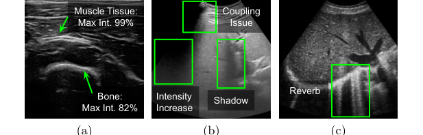 Figure 2. Complex relationship between confidence and pixel intensities. (a): tissue that blocks sound (bone) causing a weaker signal than a tissue that doesn’t block sound (muscle). (b-c): different common ultrasound artifacts
Why This Approach
The Inevitability of the Choice
The adoption of a hybrid approach, combining a physics-inspired Probabilistic Graphical Model (PGM) with a Convolutional Neural Network (CNN), was not merely an incremental improvement but a necessary paradigm shift. The authors realized that traditional "state-of-the-art" (SOTA) methods were fundamentally insufficient due to several inherent limitations. Existing approaches, often relying on simplified physical models or restricted designs, consistently failed to account for the full spectrum of ultrasound artifacts, such as reverberation, shadows, and coupling issues (Introduction, Section 2, Property 3). These methods were also hampered by arbitrary boundary conditions, which made frame-to-frame comparisons challenging and offered limited user control, requiring complex modifications to correct misassigned confidence (Introduction).
Crucially, the relationship between confidence and raw pixel intensities in ultrasound images is highly complex and non-linear (Section 2, Property 2). Simple models, whether purely physics-based or relying on basic image processing, could not adequately capture this intricate dependency. This realization highlighted the need for a learning-based component capable of discerning these subtle patterns. Therefore, a solution that could robustly integrate domain-specific physical priors, leverage sparse user feedback, and learn complex, data-driven relationships was the only viable path forward.
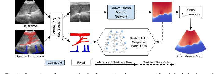 Figure 1. Overview of our method, showcasing how sparse Good (red, high confi- dence) and Bad (blue, low confidence) annotations are utilized to predict confi- dence maps with a CNN in pre-scan converted space
Comparative Superiority
This method demonstrates qualitative superiority over previous gold standards primarily through its unique hybrid architecture and user-centric design. Unlike purely physics-based models (e.g., Karamalis et al. [12]) or those focused on speckle reduction and simple propagation (e.g., Hung et al. [11]), this approach structurally addresses the multifaceted nature of ultrasound confidence.
The key structural advantage lies in the "marriage" of the PGM and the CNN. The PGM enforces fundamental ultrasound physics priors—like the mostly monotonic decay of confidence with depth (Section 3.2, Equation 4) and horizontal smoothness across scanlines (Section 3.2, Equation 5)—while also integrating sparse user annotations directly. This provides a robust, interpretable foundation. The CNN, trained on top of this PGM, then learns the complex, non-linear relationships between image intensities and confidence that simple models cannot capture (Section 3). This division of labor allows the system to be both physically grounded and highly adaptable to diverse, real-world artifacts.
Qualitatively, the method excels in handling a wide variety of challenging artifacts, including complex shadows (e.g., partial shadows, strong shadows from missing probe contact), reverberations, and unusual skin appearances caused by water baths (Section 4.1). It provides cleaner separation between visible structures and artifacts compared to competitors. Furthermore, the user-centered design, allowing practitioners to directly influence the algorithm's behavior via sparse annotations, offers an unparalleled level of control and adaptibility. The approach is also remarkably fast, exceeding 2,300 frames per second on an NVIDIA RTX 4090, making it suitable for real-time clinical applications (Section 3.3). This combination of physical grounding, learning capability, user control, and speed represents an overwhelming structural and practical advantage.
Alignment with Constraints
The chosen method perfectly aligns with the "Ideal Confidence Maps" propertys outlined in Section 2, demonstrating a thoughtful "marriage" between the problem's harsh requirements and the solution's unique properties.
- Mostly monotonic (Property 1): The
Intra-Scanline Potential$\psi_v(x_i, x_j)$ (Equation 4) within the PGM directly enforces this. It encourages confidence to mostly decrease along scanlines, penalizing deviations from this physical principle. The use of $\log(x_i)$ for penalization cleverly circumvents issues with confidence values approaching zero. - Loosely related to pixel intensities (Property 2): This is where the CNN plays a pivotal role. The paper explicitly states that the PGM does not incorporate image intensities directly due to their complex relationship with confidence. Instead, the CNN is trained to predict the most likely confidence map by minimizing the negative log-likelihood of the PGM's output, effectively learning these intricate, non-linear intensity-confidence relationships that simple models cannot capture (Section 3, Section 3.3).
- Beyond shadows (Property 3): The physics-inspired priors in the PGM, combined with the CNN's ability to learn from diverse data and sparse annotations, enable the method to handle a broad range of ultrasound artifacts—not just shadows, but also reverberations and coupling issues (Section 4.1). This comprehensive artifact handling is a direct response to the limitations of previous, more restricted models.
- Sound beams-aware (Property 4): The PGM's graph structure is designed to distinguish between intra- and inter-scanline relationships, reflecting the causal nature of sound propagation. Furthermore, inverse scan conversion is applied as a preprocessing step to ensure vertically aligned scanlines, even with non-linear fan geometries, thereby making the confidence map computation aware of the direction of insonication (Section 3, Section 3.3).
- Horizontally smooth (Property 5): The
Inter-Scanline Potential$\Psi_H(x_i, x_j)$ (Equation 5) explicitly enforces this property. By using a Gaussian function to encourage smooth transitions between adjacent scanlines, the model ensures that the confidence map reflects the physical reality of overlapping sound beams and the point-spread function.
This integrated approach ensures that the solution is not only robust and accurate but also physically plausible and user-controllable, directly addressing all the defined properties of an ideal confidence map.
Rejection of Alternatives
The paper implicitly and explicitly rejects several alternative approaches by highlighting their fundamental shortcomings in the context of ultrasound confidence map generation.
Firstly, "existing methods, relying on simplified models" (Abstract) are deemed insufficient because they "often fail to account for the full range of ultrasound artifacts and are limited by arbitrary boundary conditions" (Abstract). This broad rejection encompasses approaches that might oversimplify the complex physics of ultrasound or rely on rigid assumptions.
More specifically, the paper evaluates against and thus implicitly rejects purely physics-based graph models, such as Karamalis et al. [12]. While Karamalis' method uses graph nodes and edge weights derived from ultrasound physics, it computes confidence by solving a random walk problem with fixed boundary conditions. The authors demonstrate that this approach "poorly managed" shadows and "mistakenly assigned low confidence" to visible structures (Section 4.1). The lack of a learning component to capture complex pixel intensity relationships and the reliance on fixed boundary conditions limit its adaptibility and accurracy across diverse artifact types.
Similarly, methods like Hung et al. [11], which reduce speckle and propagate confidence using directed acyclic graphs, are shown to struggle with various artifacts, particularly shadows, and often misassign low confidence to visible structures (Section 4.1). These methods, while perhaps addressing some aspects like speckle, lack the comprehensive artifact handling and user-controllability of the proposed hybrid model.
The paper also mentions "shadow-based models [15] are restricted by design" (Introduction) and explicitly excludes them from quantitative comparison due to the lack of shadow-specific annotations (Section 4). This highlights the limitation of approaches that are too specialized, failing to generalize across the broad range of artifacts present in real-world ultrasound.
Finally, Ultra-NeRF based approaches [22,23] were not included in the qualitative evaluation due to their "requirement of perfectly aligned ultrasound and CT volumes for the training phase" (Section 4.2). This points to a practical constraint that makes such methods less suitable for scenarios where such perfectly aligned multi-modal data might not be readily available, underscoring the importance of a method that can work with more accessible sparse annotations.
In essence, the rejection of these alternatives stems from their inability to simultaneously: 1) account for the full range of ultrasound artifacts, 2) capture the complex, non-linear relationship between pixel intensities and confidence, 3) offer user control, and 4) maintain temporal stability and real-time performance. The proposed PGM-CNN hybrid was developed to overcome these collective failings.
Mathematical & Logical Mechanism
The Master Equation
At the heart of this paper's mechanism lies a two-pronged mathematical engine. The first part defines the probabilistic graphical model (PGM) that quantifies the likelihood of a confidence map given sparse user annotations and physics-inspired priors. The second part is the objective function that drives the learning of the Convolutional Neural Network (CNN) by minimizing the negative log-likelihood derived from this PGM.
The core probabilistic model, defining the likelihood of a confidence map $x$ given sparse annotations $y$, is:
$$
p(x|y) \propto \prod \phi(x_i, y_i) \prod_{(i,j)\in V} \psi_V(x_i, x_j) \prod_{(i,j)\in H} \psi_H(x_i, x_j) \quad (2)
$$
And the ultimate objective function that the CNN optimizes is:
$$
\theta^* = \arg \min_\theta - \log p(f(I^{(i)}, \theta), y^{(i)}) \quad (6)
$$
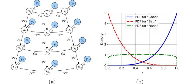 Figure 3. (a) Graphical representation of the PGM used to combine sparse anno- tations with a physics based prior. Refer to the text for the description of the pairwise potentials ϕ , ψV , ψH. (b) Plot of the Probability Density Functions (PDF) for the Beta distributions used in the definition of ϕ
Term-by-Term Autopsy
Let's dissect these equations to understand every component:
Equation (6): The Optimization Objective
- $\theta^*$:
- Mathematical Definition: The optimal set of parameters for the Convolutional Neural Network (CNN).
- Physical/Logical Role: This is the ultimate goal of the learning process. It represents the specific configuration of weights and biases within the CNN that allows it to generate the most plausible confidence maps according to the defined probabilistic model.
- $\arg \min_\theta$:
- Mathematical Definition: The argument (in this case, the parameters $\theta$) that minimizes the subsequent expression.
- Physical/Logical Role: This operator signifies that the learning algorithm is searching for the CNN parameters that yield the smallest possible value for the loss function.
- $-\log$:
- Mathematical Definition: The negative natural logarithm.
- Physical/Logical Role: This transformation serves two key purposes. First, it converts a probability (which is between 0 and 1) into a positive value, making it suitable for minimization (as minimizing negative log-likelihood is equivalent to maximizing likelihood). Second, it transforms products of probabilities (or potentials, as seen in Equation 2) into sums, which are much easier to differentiate during the backpropagation process.
- Why: Logarithms are chosen because they simplify the product structure of the PGM into a sum, which is computationally more stable and easier for gradient-based optimization. The negative sign flips the problem from maximization to minimization.
- $p(\cdot)$:
- Mathematical Definition: A probability distribution.
- Physical/Logical Role: This term represents the likelihood of a predicted confidence map, as defined by the Probabilistic Graphical Model (PGM) in Equation (2). It quantifies how compatible the CNN's output is with both the user annotations and the physics-inspired priors.
- $f(I^{(i)}, \theta)$:
- Mathematical Definition: The output of the Convolutional Neural Network $f$ when given an input ultrasound image $I^{(i)}$ and current parameters $\theta$.
- Physical/Logical Role: This is the CNN's prediction: a confidence map $x$ for the $i$-th ultrasound image. The CNN is trained to produce these maps, which are then evaluated by the PGM.
- $y^{(i)}$:
- Mathematical Definition: The sparse binary annotations provided for the $i$-th ultrasound image.
- Physical/Logical Role: These are the ground truth or user-provided labels (Good, Bad, or None) that serve as supervision for the learning process. They anchor the confidence map to human expert knowledge.
Equation (2): The Probabilistic Graphical Model
- $p(x|y)$:
- Mathematical Definition: The probability of a confidence map $x$ given sparse annotations $y$.
- Physical/Logical Role: This is the core of the PGM. It provides a quantitative measure of how likely a particular confidence map $x$ is, considering both the user's input $y$ and the embedded physics-inspired rules.
- $\propto$:
- Mathematical Definition: Proportional to.
- Physical/Logical Role: This indicates that the expression on the right-hand side is proportional to the true probability. There's an implicit normalization constant (often called the partition function) that makes the probabilities sum to 1. For optimization purposes, this constant can often be ignored as it doesn't affect the relative likelihoods.
- $\prod$:
- Mathematical Definition: The product operator.
- Physical/Logical Role: In a graphical model, the joint probability is typically expressed as a product of potential functions over cliques (groups of interconnected nodes). Here, it combines the individual unary and pairwise potentials multiplicatively to form the overall likelihood.
- Why: This multiplicative structure is fundamental to Markov Random Fields and other PGMs, where potentials represent local "agreements" or "compatibilities" that combine to form a global probability.
- $\phi(x_i, y_i)$:
- Mathematical Definition: The unary potential function for pixel $i$.
- Physical/Logical Role: This term measures the compatibility between the predicted confidence value $x_i$ for a specific pixel and its corresponding sparse annotation $y_i$. It directly enforces the user's input on individual pixels.
- Why: The product combines the individual compatibilities of each annotated pixel.
- $\prod_{(i,j)\in V}$:
- Mathematical Definition: Product over all vertically adjacent pixel pairs $(i,j)$.
- Physical/Logical Role: This operator aggregates the intra-scanline pairwise potentials, ensuring that the physics-inspired prior for vertical relationships is applied across the entire confidence map.
- $\psi_V(x_i, x_j)$:
- Mathematical Definition: The vertical (intra-scanline) pairwise potential function (defined in Equation 4).
- Physical/Logical Role: This potential enforces the "mostly monotonic" property (Property 1) along scanlines. It penalizes situations where confidence does not decrease sufficiently with depth, reflecting the physical attenuation of ultrasound signals.
- Why: The product combines these vertical relationship compatibilities.
- $\prod_{(i,j)\in H}$:
- Mathematical Definition: Product over all horizontally adjacent pixel pairs $(i,j)$.
- Physical/Logical Role: This operator aggregates the inter-scanline pairwise potentials, ensuring that the physics-inspired prior for horizontal relationships is applied across the entire confidence map.
- $\psi_H(x_i, x_j)$:
- Mathematical Definition: The horizontal (inter-scanline) pairwise potential function (defined in Equation 5).
- Physical/Logical Role: This potential enforces the "horizontally smooth" property (Property 5) between scanlines. It encourages similar confidence values for adjacent pixels in the horizontal direction, reflecting the overlap of ultrasound beams and the continuous nature of tissue.
- Why: The product combines these horizontal relationship compatibilities.
Equation (3): Unary Potential Details
- $\text{Beta}(z; \alpha, \beta)$:
- Mathematical Definition: The Probability Density Function (PDF) of the Beta distribution.
- Physical/Logical Role: The Beta distribution is ideal for modeling probabilities or confidence values that are bounded between 0 and 1. Its shape parameters $\alpha$ and $\beta$ allow it to be peaked at different values, representing different levels of confidence.
- Why: It's a natural choice for modeling confidence values, which are inherently probabilities.
- $x_i$:
- Mathematical Definition: The confidence value for pixel $i$.
- Physical/Logical Role: This is the specific confidence score (between 0 and 1) that the CNN has predicted for a given pixel.
- $y_i$:
- Mathematical Definition: The annotation for pixel $i$.
- Physical/Logical Role: This is the user's label for pixel $i$, which can be 'Good' (high confidence), 'Bad' (low confidence), or 'None' (unannotated).
- $\alpha, \beta$:
- Mathematical Definition: Shape parameters of the Beta distribution.
- Physical/Logical Role: These parameters dictate the shape of the Beta distribution. For 'Good' annotations ($\alpha=5, \beta=1$), the distribution is heavily peaked towards 1, strongly favoring high confidence. For 'Bad' annotations, applying $\text{Beta}(1-x_i; \alpha=5, \beta=1)$ means the distribution for $x_i$ is peaked towards 0, favoring low confidence. For 'None' annotations ($\alpha=1.1, \beta=1.1$), the distribution is flatter, indicating a weaker preference for extreme confidence values, allowing pairwise potentials to have more influence.
- Why: These specific values are empirically chosen to reflect the desired probability distributions for each annotation type, as visualized in Figure 3b.
Equation (4): Vertical Pairwise Potential Details
- $\exp(\cdot)$:
- Mathematical Definition: The exponential function.
- Physical/Logical Role: This converts the penalty term (which is in the exponent) into a potential value. A larger penalty (more negative exponent) results in a smaller potential, indicating lower compatibility.
- $-\gamma$:
- Mathematical Definition: A negative scaling factor.
- Physical/Logical Role: $\gamma$ is a parameter that controls the strength of this prior. A larger $\gamma$ means a stronger penalty for violating the monotonic decrease of confidence along a scanline.
- $\max(0, \cdot)$:
- Mathematical Definition: The maximum of 0 and the argument.
- Physical/Logical Role: This ensures that a penalty is only applied when the condition for monotonic decrease is violated. If $x_j$ decreases as expected or more, there is no penalty (the term becomes 0, and $\exp(0)=1$, meaning no reduction in potential).
- $\log(x_j) - \log(x_i)$:
- Mathematical Definition: The difference of natural logarithms, equivalent to $\log(x_j/x_i)$.
- Physical/Logical Role: This term measures the relative change in confidence between pixel $i$ and pixel $j$. Using logarithms addresses a limitation of direct confidence values: when $x_i$ is already very low, it cannot decrease much further, making it hard to penalize. Logarithms are not bounded below, allowing for consistent penalty application.
- $s$:
- Mathematical Definition: A constant parameter.
- Physical/Logical Role: This parameter represents the desired decay in confidence between adjacent pixels along a scanline. It acts as a threshold: if $\log(x_j) - \log(x_i)$ is greater than $-s$, it means $x_j$ hasn't decreased enough relative to $x_i$, incurring a penalty.
- Why: The authors chose $\log(x)$ to overcome the "zero-bound" issue of confidence values, ensuring that the monotonic decay prior can be applied effectively even at low confidence levels.
Equation (5): Horizontal Pairwise Potential Details
- $\exp(\cdot)$:
- Mathematical Definition: The exponential function.
- Physical/Logical Role: Similar to $\psi_V$, this converts the squared difference penalty into a potential. Larger differences lead to smaller potentials.
- $-\sigma$:
- Mathematical Definition: A negative scaling factor.
- Physical/Logical Role: $\sigma$ is a parameter controlling the strength of this prior. A larger $\sigma$ means a stronger penalty for differences between horizontally adjacent pixels, thus encouraging greater smoothness.
- $(x_i - x_j)^2$:
- Mathematical Definition: The squared difference between the confidence values of horizontally adjacent pixels $i$ and $j$.
- Physical/Logical Role: This term quantifies the dissimilarity or lack of smoothness between $x_i$ and $x_j$. Squaring ensures the penalty is always positive and that larger deviations are penalized more significantly.
- Why: The squared difference is a standard and effective way to penalize deviations from a desired state (here, smoothness). The negative exponential creates a Gaussian-like potential, where pixels with very similar confidence values yield high potentials, while dissimilar ones yield low potentials.
Step-by-Step Flow
Imagine a single ultrasound image, $I^{(i)}$, entering this system like a raw material on an assembly line. Here's how it's processed to generate and refine a confidence map:
- Initial Prediction (CNN Stage): The raw ultrasound image $I^{(i)}$ is first fed into the Convolutional Neural Network, $f(\cdot, \theta)$. This CNN, acting as the initial processing unit, transforms the image into a preliminary confidence map, $x = f(I^{(i)}, \theta)$. Each pixel $x_k$ in this map represents the network's initial guess of confidence, a value typically between 0 and 1.
- Annotation Compatibility Check (Unary Potentials): Next, for each individual pixel $x_k$ in the predicted confidence map, the system checks if there's a corresponding sparse annotation $y_k$ provided by a user. If an annotation exists (Good, Bad, or None), a "unary potential" $\phi(x_k, y_k)$ is calculated using a Beta distribution. This step acts like a quality control station, measuring how well the CNN's predicted confidence $x_k$ aligns with the human expert's label $y_k$. A high potential means good alignment.
- Vertical Physics Enforcement (Intra-Scanline Potentials): Simultaneously, the system examines pairs of vertically adjacent pixels $(x_i, x_j)$ along each scanline. A "vertical pairwise potential" $\psi_V(x_i, x_j)$ is computed. This mechanism acts as a physics-inspired regulator, ensuring that confidence generally decreases as depth increases, reflecting the natural attenuation of ultrasound signals. If confidence unexpectedly increases or doesn't decrease enough, this potential imposes a penalty, reducing the overall likelihood.
- Horizontal Smoothness Enforcement (Inter-Scanline Potentials): In parallel, the system also looks at pairs of horizontally adjacent pixels $(x_i, x_j)$ across different scanlines. A "horizontal pairwise potential" $\psi_H(x_i, x_j)$ is calculated. This component acts like a smoothing filter, encouraging neighboring pixels across scanlines to have similar confidence values. This reflects the physical reality of overlapping ultrasound beams and continuous tissue properties, penalizing abrupt horizontal changes.
- Global Likelihood Assembly (PGM Integration): All these individual compatibility scores – the unary potentials from annotations, the vertical potentials from physics, and the horizontal potentials from smoothness – are then multiplied together. This multiplication, as defined in Equation (2), yields a single, comprehensive likelihood score $p(x|y)$ for the entire predicted confidence map $x$. This score represents how "plausible" the CNN's output map is, considering all the guiding principles.
- Loss Calculation (Negative Log-Likelihood): Finally, this global likelihood $p(x|y)$ is transformed by taking its negative logarithm, resulting in $-\log p(x|y)$. This value is the "loss" for the current input image. It's the metric that the system aims to minimize, effectively turning the problem of finding the most likely confidence map into a standard optimization challenge for the CNN.
This entire process is repeated for many images, allowing the CNN to learn from the feedback provided by the PGM.
Optimization Dynamics
The mechanism learns, updates, and converges through a process of iteratively refining the CNN's parameters ($\theta$) to minimize the negative log-likelihood defined by the Probabilistic Graphical Model.
-
Loss Landscape Shaping: The PGM plays a crucial role in shaping the loss landscape for the CNN. Instead of a simple pixel-wise loss, the PGM creates a sophisticated landscape with "valleys" that correspond to confidence maps that are not only consistent with sparse user annotations but also adhere to fundamental ultrasound physics principles.
- Unary Potentials: These act as strong attractors. If a pixel is annotated 'Good', the loss landscape will have a steep slope pushing the CNN's output $x_i$ towards 1. If 'Bad', it pushes $x_i$ towards 0. For 'None' annotations, the landscape is flatter, allowing the pairwise potentials to guide the confidence value.
- Vertical Pairwise Potentials: These introduce a directional bias. The landscape becomes steeper (higher loss) for confidence maps where values increase with depth or do not decrease sufficiently, effectively creating a "downhill" slope for confidence along scanlines.
- Horizontal Pairwise Potentials: These enforce smoothness. The landscape will have deep, narrow valleys where horizontally adjacent pixels have very similar confidence values, penalizing sharp discontinuities and encouraging smooth transitions.
- The negative logarithm ensures that even small deviations from highly probable configurations result in a significant increase in loss, providing strong gradients for learning.
-
Gradient Descent and Backpropagation: The CNN learns using an iterative optimization algorithm, typically a variant of stochastic gradient descent (e.g., Adam).
- During each training step, a batch of ultrasound images is fed into the CNN, which produces a batch of predicted confidence maps.
- For each predicted map, the PGM calculates the negative log-likelihood loss, as described in the "Step-by-Step Flow."
- Backpropagation is then used to compute the gradients of this loss with respect to every parameter $\theta$ within the CNN. These gradients indicate the direction and magnitude of change needed for each parameter to reduce the loss.
- The optimizer then updates the CNN's parameters by taking a step in the opposite direction of the gradient (down the loss landscape), scaled by a learning rate. This iterative adjustment allows the CNN to gradually learn the complex mapping from ultrasound images to confidence maps that satisfy the PGM's criteria.
-
Convergence Behavior: The combination of a powerful CNN and a physics-informed PGM facilitates robust convergence.
- The PGM acts as a strong, interpretable prior, guiding the CNN towards physically plausible solutions and preventing it from getting stuck in local minima that might satisfy sparse annotations but violate fundamental physics. This is a key advantage over purely data-driven approaches.
- The authors report a validation loss of 0.32, closely matching the training loss of 0.25. This indicates that the model is learning effectively and generalizing well to unseen data, without significant overfitting. The PGM's regularization effect likely contributes to this good generalization.
- The iterative updates continue until the gradients become very small, indicating that the model has reached a stable point in the loss landscape where further parameter adjustments yield minimal improvement. This results in a CNN capable of rapidly generating high-quality, physics-consistent confidence maps in real-time.
Results, Limitations & Conclusion
Experimental Design & Baselines
To rigorously validate their novel approach, the authors architected a series of experiments, pitting their physics-inspired, CNN-driven confidence map generation against established methods. The "victims" (baseline models) in this comparative analysis were primarily the methods proposed by Karamalis et al. [12] and Hung et al. [11].
Karamalis' method operates by modeling image pixels as nodes in a graph, where edge weights are derived from ultrasound physics. Confidence is then computed by solving a random walk equilibrium problem, constrained by fixed boundary conditions (high confidence at the top, low at the bottom). For a fair comparison, the authors utilized a publicly available Python implementation of this method, setting its alpha parameter to 1. Hung's approach, on the other hand, first reduces speckle noise using an anisotropic filter and then propagates confidence downwards from the image's top row via a directed acyclic graph. The authors used the official implementation of Hung's method, carefully setting its parameters ($\alpha = 10^{-2}$ and $\xi = 0.4$) to prevent overly rapid confidence decay. Notably, a shadow-specific neural network approach [15] was excluded from the comparison due to the lack of necessary shadow annotations in the available datasets.
The experimental design encompassed both qualitative and quantitative evaluations across diverse ultrasound scenarios:
-
Qualitative Evaluation: A set of seven representative ultrasound frames (A-G) from the validation dataset was chosen. Frames A-F were acquired under similar conditions to the training data, while Frame G was deliberately selected from a completely different setup—involving a different ultrasound machine and a water bath for acoustic coupling—to test the generalization capabilities of the proposed method. This allowed for a visual assessment of how well each method handled various artifacts and imaging conditions.
-
Quantitative Evaluation: Bone Shadow Segmentation: This task built upon the prior work of Yesilkaynak et al. [23]. The authors leveraged Yesilkaynak's publicly available code and dataset, which includes ultrasound frames and corresponding bone shadow masks. To ensure an unbiased comparison, their proposed confidence estimation was applied to all frames, and then a random forest classifier (without any modifications or finetuning) was used to predict shadows. This setup ensured that any performance differences were solely attributable to the quality of the generated confidence maps, not to task-specific optimization of the segmentation algorithm itself.
-
Quantitative Evaluation: Registration Weighting: For a second downstream task, the authors followed the evaluation methodology from Ronchetti et al. [16]. The dataset for this task comprised 28 tracked liver clips from two different ultrasound machines, with positional information obtained via optical tracking. Each clip was paired with a corresponding CT or MR volume, and at least four landmark pairs were manually annotated by an expert. Individual confidence maps were computed for all frames, which were then used to reconstruct a 3D confidence volume. Experiments were conducted using the confidence maps directly as weighting factors for multi-modal intensity-based registration, and also by multiplying them with local patch variance, replacing the conventional use of patch variance alone. This allowed for a direct assessment of how the confidence maps improved the robustness and convergence of registration algorithms.
What the Evidence Proves
The evidence presented in the paper provides a compelling case for the efficacy and superiority of the proposed physics-inspired learning approach for ultrasound confidence maps. The core mechanism, which integrates sparse annotations into a probabilistic graphical model (PGM) to guide a convolutional neural network (CNN), demonstrably works in reality, outperforming baselines across various challenging scenarios.
Qualitative Evidence (Figure 4):
The visual comparison in Figure 4 offers undeniable proof of the method's robustness. The proposed approach consistently generates more accurate and intuitive confidence maps compared to Karamalis' and Hung's methods, particularly in the presence of complex artifacts:
* Shadow Handling: The method excels at identifying and delineating shadows, which are often poorly managed by the baselines. For instance, in Frame B, a partial shadow followed by a strong reflector (diaphragm) is correctly detected by our method, which also assigns an appropriate intermediate confidence to the diaphragm. In contrast, other methods completely miss this nuanced shadow. Similarly, strong shadows caused by missing probe contact (Frames A and E) are entirely mistaken by the competing approaches, highlighting a critical failure in their ability to interpret these common artifacts.
* Reverberation and Artifact Separation: While Hung's method shows some capability in dealing with reverberation (Frames A, F), our approach provides a much cleaner separation between visible structures and artifacts, leading to more reliable confidence assessments.
* Preservation of High Confidence: Crucially, the proposed method avoids mistakenly assigning low confidence to visible structures at higher depths (Frames C, D, G), a common pitfall for Karamalis' and Hung's methods.
* Generalization: The performance on Frame G, acquired with a completely different ultrasound machine and a water bath (not part of the training data), is particularly striking. Our method correctly recognizes the unusual skin appearance and artifacts, demonstrating strong generalization capabilities beyond the training distribution. This is a powerful testament to the underlying physics-inspired prior and the CNN's ability to learn robust features.
 Figure 4. Ultrasound frames (before scan conv.), with confidence maps generated by three methods. Red and blue represent high and low confidence, respectively. The squares on the confidence maps show regions of interest. See text for details
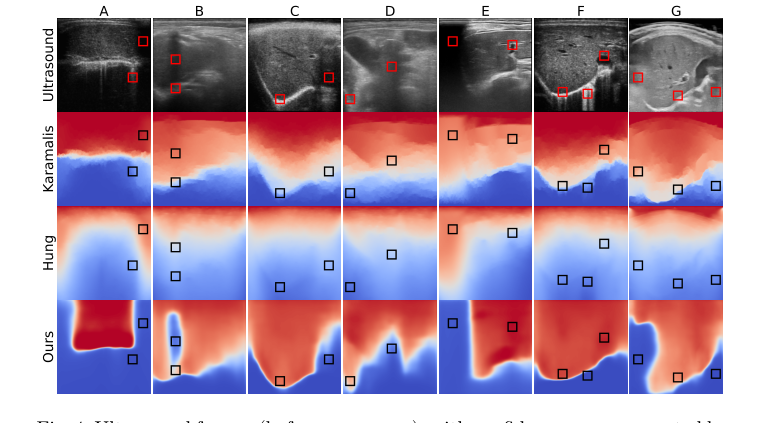 Figure 4. depicts 7 representative frames (A-G), selected from the validation set. While Frames A-F were acquired with the same setups as our training data, Frame G comes from a completely different setup, demonstrating the general- ization capabilities of our approach. Specifically, Frame G was acquired with a different ultrasound machine and through a water bath for optimized acoustic coupling, which causes the unusual artifacts visible on the left of the frame. Our
Quantitative Evidence (Bone Shadow Segmentation - Table 1):
The quantitative results for bone shadow segmentation provide hard numbers that underscore the qualitative observations. Without any task-specific finetuning or objective in its training, the proposed method significantly outperforms the state-of-the-art:
* Dice Score: Our method achieved a Dice score of 58.9%, which is substantially higher than Yesilkaynak (50.4%), Karamalis (49.3%), and Hung (47.6%). A higher Dice score indicates better overlap between the predicted and ground truth shadow regions.
* Precision: The precision of our method was 86.8%, far exceeding Yesilkaynak (71.5%), Hung (63.4%), and Karamalis (61.1%). This metric confirms that when our method identifies a shadow, it is highly likely to be correct, minimizing false positives.
* Hausdorff Distance: While Yesilkaynak's method had a slightly better Hausdorff distance (5.6 vs. 6.2 for ours), the overall superior performance in Dice score and precision definitively proves that our confidence maps are more effective for this downstream task.
Quantitative Evidence (Registration Weighting - Table 2):
The second quantitative evaluation, focusing on multi-modal registration, further solidifies the claims. The confidence maps generated by the proposed method significantly improve the convergence rate of registration algorithms:
* Increased Converged Cases: Across all categories of initial registration error (<25mm, 25-50mm, >50mm), "Ours" and "Ours × Variance" consistently yielded the highest percentage of converged cases. For initial errors less than 25mm, our method achieved 77.9% convergence (and 78.7% when combined with variance), dramatically surpassing the baseline "Variance" (69.7%), Karamalis (31.1%), and Hung (49.4%). Even when baselines were combined with variance (e.g., Karamalis × Variance at 70.4%), our method still showed a clear advantage.
* This demonstrates that the confidence maps provide a more reliable and robust weighting factor for registration, leading to more successful and stable alignments between ultrasound and CT/MR volumes. The ability to support registration convergence in a significantly higher number of cases is a critical clinical advantage.
In summary, the experimental results, both visual and numerical, provide definitive, undeniable evidence that the proposed user-centered, physics-inspired approach generates superior ultrasound confidence maps that are robust to artifacts, generalize well, and significantly enhance performance in downstream tasks like bone shadow segmentation and multi-modal image registration.
Limitations & Future Directions
While the proposed method marks a significant advancement in generating robust ultrasound confidence maps, it's important to acknowledge its current limitations and consider avenues for future development. The paper itself points to a few areas, and a broader perspective can stimulate further critical thinking.
One inherent limitation, as noted in Section 2, is that the underlying physical model for ideal confidence maps does not explicitly account for complex phenomena like multi-path scattering or reverberation. While the CNN is trained to implicitly handle these artifacts, a more direct integration of such physics into the probabilistic graphical model (PGM) could potentially enhance robustness and reduce reliance on extensive training data. Similarly, the PGM does not directly use image intensities, instead delegating this complex relationship to the CNN. While this design choice was intentional, it raises questions about whether a more sophisticated, physics-informed integration of intensity data within the PGM itself could yield even more precise confidence estimations, especially in ambiguous regions.
Another practical limitation, though not explicitly stated as such, is the current focus on 2D ultrasound frames. While the method is shown to be fast enough for real-time applications, clinical workflows often require volumetric analysis. The paper's conclusion mentions extending the approach to 3D ultrasound for volumetric analysis as future work, which is a natural and necessary progression.
Looking ahead, several discussion topics emerge for further developing and evolving these findings:
-
Deepening Physics-Informed Learning: How can we move beyond the current physics-inspired prior to a truly physics-constrained or physics-regularized learning framework? Could differentiable physics simulators be integrated into the training loop to provide richer, more accurate priors, potentially reducing the need for large annotated datasets and improving generalization to unseen artifacts or transducer types? This could involve modeling more complex wave propagation phenomena, such as non-linear acoustics or tissue-specific attenuation profiles.
-
Adaptive and Active Annotation Strategies: The current method relies on sparse binary annotations. While effective, the process of obtaining these annotations can still be labor-intensive. Future work could explore active learning frameworks where the model intelligently identifies regions of high uncertainty or disagreement and requests targeted annotations from experts. This could optimize the annotation effort, focusing human input where it provides the most value, and potentially lead to more efficient model training and adaptation to new clinical scenarios.
-
Uncertainty Quantification of Confidence Maps: While the method generates confidence maps, it doesn't explicitly quantify the uncertainty of these confidence maps themselves. In high-stakes clinical decisions, knowing how certain the model is about its confidence prediction could be invaluable. Exploring Bayesian neural networks, ensemble methods, or other uncertainty quantification techniques could provide a "confidence in confidence" metric, offering clinicians a more complete picture of image reliability.
-
Real-time Clinical Integration and Feedback Loops: The reported speed of 2,300 fps makes this method highly suitable for real-time clinical use. The next frontier is seamless integration into existing ultrasound machines and clinical workflows. Beyond simply displaying the confidence map, how can clinicians provide real-time, intuitive feedback (e.g., through gestures, voice commands, or direct manipulation) to continuously refine the model's behavior in a live setting? This could lead to truly personalized and adaptive confidence mapping systems that learn from ongoing clinical experience.
-
Multi-modal and Multi-source Confidence Fusion: The paper demonstrates the utility of confidence maps for multi-modal registration. This concept could be expanded to fuse confidence information from multiple sources—not just different imaging modalities (e.g., combining ultrasound confidence with CT-derived anatomical certainty) but also from different ultrasound acquisition parameters or even different operators. A composite confidence map, leveraging the strengths of various inputs, could offer a more robust and comprehensive assessment of image quality.
-
Beyond Current Downstream Tasks: The method has shown promise in bone shadow segmentation and registration. What other critical downstream tasks in medical imaging could benefit significantly from these high-quality confidence maps? Potential applications include automated lesion detection and characterization, guiding robotic interventions (e.g., biopsy, ablation) where precise knowledge of tissue reliability is paramount, or even improving the training of other deep learning models by weighting their loss functions based on image confidence.
-
Ethical Considerations and Trust in AI: As AI-driven confidence maps become more integrated into clinical decision-making, ethical considerations become paramount. How do we ensure that clinicians develop appropriate trust in these systems, avoiding both over-reliance and undue skepticism? Research into explainable AI (XAI) for confidence maps could help elucidate why certain regions are deemed high or low confidence, fostering transparency and building clinician confidence in the tool itself. This is a crucial aspect for successful clinical adoption.
The journey "Beyond Shadows" is clearly just beginning, and these findings lay a solid foundation for a future where ultrasound imaging is not only real-time but also reliably quantified, empowering clinicians with better information for diagnosis and intervention.
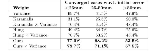 Table 2. Impact of using confidence as voxel weight for registration. A case is considered “converged” if the Fiducial Registration Error after registration is below 15 mm. The best results and the ones not significantly different (p > 10−3) are highlighted in bold
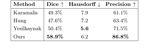 Table 1. Random forest shadow segmentation using confidence maps. All rows except the last one are reprinted from [23], see text for details