Global exponential stability analysis for a delayed diffusive Nicholson’s blowflies equation
A modified Nicholson’s blowflies equation accompanying distinct time-varying delays is established in this paper.
Background & Academic Lineage
The Origin & Academic Lineage
The problem addressed in this paper originates from the field of mathematical biology, specifically in the modeling of population dynamics. Historically, simple models like the logistic equation were used to describe population growth. However, real-world biological populations often exhibit more complex behaviors, particularly due to time delays in life cycles and spatial movement.
The specific problem of analyzing Nicholson's blowflies equation emerged as researchers sought to create more realistic models for insect populations, where factors like maturation time significantly influence population size. Blowflies, in particular, have been a classic subject for such studies due to their distinct life stages and the observable impact of delayed maturation on population fluctuations. The original Nicholson's blowflies equation is a delay differential equation that captures the oscillatory behavior often seen in populations with delayed feedback mechanisms.
This paper builds upon previous work, notably reference [4], which introduced a modified diffusive Nicholson's blowflies model (Equation 1.1) that incorporates both spatial diffusion and multiple time-varying delays. The "diffusive" aspect accounts for the spatial spread of mature individuals, while "time-varying delays" reflect that maturation periods might not be constant but change over time due to environmental factors.
The fundamental limitation or "pain point" of previous approaches, and the primary motivation for this paper, lies in the inability of classical dynamical systems theory to analyze the stability of the positive steady state under certain conditions. Specifically, earlier work, including [4], successfully established the stability of the zero steady state (i.e., population extinction) when the reproduction rate was low ($\sum_{j=1}^m \frac{\beta_j}{\gamma} \leq 1$). However, when the reproduction rate was high ($\sum_{j=1}^m \frac{\beta_j}{\gamma} > 1$), and thus a positive steady state (a stable, non-zero population level) was expected, classical theory failed. This failure was due to the complex nature of non-autonomous equations with time-varying delays, which typically lack a "semi-flow structure" that is crucial for traditional stability analysys. This theoretical obstacle was explicitly identified as an open problem in the concluding remarks of [4], and it remained unresolved until this paper. The authors were compelled to write this paper to overcome this limitation and provide a rigorous framework for understanding the global exponential stability of the positive steady state in these more realistic and complex models.
Intuitive Domain Terms
- Nicholson's blowflies equation: Imagine a mathematical "story" that describes how a group of blowflies grows and shrinks over time. This story includes rules for how many new flies are born, how many die, and crucially, how long it takes for a baby fly to become an adult. It's a specific formula designed to mimic the real-life ups and downs of a blowfly population.
- Time-varying delays: Think about the time it takes for a seed to grow into a flower. This "delay" isn't always the same; it might be shorter in warm, sunny weather and longer in cold, cloudy conditions. In the blowflies model, "time-varying delays" mean that the time it takes for a blowfly to mature isn't fixed but changes dynamically, making the model more true to life.
- Diffusive: Picture a drop of food coloring spreading out in a glass of water. "Diffusive" in this context means that the blowflies don't just stay in one spot; they move and spread out across their habitat. This spatial movement is an important part of how their population changes over an area.
- Global exponential stability: This is like a self-righting toy. No matter how you push it or where you start it from, it will always quickly and smoothly return to its upright, stable position. "Global" means it works from any starting point, and "exponential" means it settles into that stable position very efficiently and rapidly, like a fast-dampening oscillation, reaching its equillibrium.
Notation Table
| Notation | Description |
|---|---|
| $\Theta(t,x)$ | The population density of blowflies at time $t$ and spatial location $x$. |
| $M$ | A bounded spatial domain in $\mathbb{R}^N$ with a smooth boundary $\partial M$. |
| $\Delta$ | The Laplacian operator, representing spatial diffusion. |
| $\gamma$ | The per capita daily mortality rate of adult blowflies ($\gamma > 0$). |
| $m$ | The number of distinct groups of blowflies, each with its own delay and density-dependent parameters. |
| $\beta_j$ | The per capita daily spawn production coefficient for group $j$ ($\beta_j > 0$). |
| $r_j(t)$ | The time-varying maturation delay for group $j$ ($r_j(t) > 0$). |
| $a_j$ | The density-dependent intensity parameter for group $j$ ($a_j > 0$). |
| $e^{-a_j \Theta(t - r_j(t), x)}$ | The exponential term modeling density-dependent self-limitation during the immature stage. |
| $\frac{\partial \Theta}{\partial n}(t,x) = 0$ | Neumann boundary condition, indicating no-flux across the boundary $\partial M$. |
| $\psi(\theta, x)$ | The initial history function for the population density over the interval $[-\tau, 0] \times M$, where $\tau = \max_j \tau_j$ is the maximum delay. |
| $X_+$ | The space of non-negative continuous functions, representing biologically realistic population densities. |
| $\Theta^*$ | The unique positive steady state solution of the equation, representing a stable, non-zero equilibrium population density. |
| $A = \Delta - \gamma Id$ | The linear operator representing diffusion and mortality, where $Id$ is the identity operator. |
| $T(t)$ | The strongly continuous semigroup of linear operators generated by the closure of $A$ under Neumann boundary conditions. |
| $\kappa^*$ | A specific constant in $(0,1)$ crucial for stating global exponential stability results. |
| $\sum_{j=1}^m \frac{\beta_j}{\gamma}$ | A key parameter representing the total reproduction rate relative to mortality, influencing the existence and stability of steady states. |
| $\sum_{j=1}^m \frac{\beta_j}{a_j \gamma}$ | Another key parameter, particularly relevant for the stability of the zero steady state. |
| $\sum_{j=1}^m \frac{\beta_j}{\gamma} e^{-a_j \Theta^*}$ | A condition derived from the characteristic equation of the steady state, used to determine its stability. |
| $\lambda$ | A positive constant representing the exponential decay rate in global exponential stability. |
| $N_0$ | A positive constant representing the initial bound for exponential attractivity. |
| $l, L$ | Lower and upper bounds for the solution $B(t)$ in the fluctuation lemma. |
| $z^0$ | A positive constant used in the proof of Lemma 2.3 for lower bounds of solutions. |
| $\delta_0$ | A small positive constant used in the proof of Lemma 2.4. |
| $\xi$ | A time threshold after which solutions are bounded within a certain range. |
| $b^*$ | An upper bound for the solution $\Theta^0(t,x)$ after time $\xi$. |
Problem Definition & Constraints
Core Problem Formulation & The Dilemma
The core problem addressed in this paper revolves around understanding the long-term behavior of a biological population model. Specifically, the authors are investigating a modified diffusive Nicholson's blowflies equation, presented as initial boundary value problem (IBVP) (1.1), which incorporates multiple time-varying delays and a Neumann boundary condition.
The starting point (Input/Current State) is the existence of this complex mathematical model, which aims to more accurately represent real-world population dynamics by including factors like diffusion and time-dependent maturation delays. Previous research, notably [4], had already established criteria for the stability and global exponential attractivity of the zero steady state solution for this model under specific conditions (e.g., $\sum_{j=1}^m \frac{\beta_j}{\gamma} \le 1$ and $\sum_{j=1}^m \frac{\beta_j}{a_j \gamma} < 1$). This means that under those conditions, the population would eventually die out.
The desired endpoint (Output/Goal State) is to determine the conditions under which the positive steady state solution ($\Theta^*$) of IBVP (1.1) exhibits global exponential stability and attractivity. This is crucial for understanding how a population can persist and stabilize at a non-zero level. The paper specifically targets the scenario where $\sum_{j=1}^m \frac{\beta_j}{a_j \gamma} > 1$, a condition under which the zero steady state is unstable, implying the potential for a positive equilibrium.
The exact missing link or mathematical gap is the absence of a robust theoretical framework to analyze the stability and exponential attractivity of this positive steady state when the model includes non-autonomous equations with time-varying delays. This particular configuration typically lacks a semi-flow structure, which is a prerequisite for applying classical dynamical systems theory. This gap was explicitly identified as an open problem in the concluding remarks of [4], remaining unresolved until this work.
The painful trade-off or dilema that has trapped previous researchers is the inherent conflict between biological realism and mathematical tractability. While incorporating multiple time-varying delays ($r_j(t)$) and distinct density-dependent intensity parameters ($a_j$) makes the Nicholson's blowflies equation a more faithful representation of biological phenomena, these very features introduce significant mathematical complexities. The non-autonomous nature and time-varying delays disrupt the semi-flow structure, rendering standard analytical tools ineffective for the positive steady state. Thus, improving the model's descriptive power simultaneously made its rigorous stability analysis, particularly for a non-extinct population, exceedingly difficult.
Constraints & Failure Modes
This problem is insanely difficult to solve due to several harsh, realistic walls the authors hit, primarily stemming from the mathematical structure of the model:
- Lack of Semi-flow Structure (Mathematical Constraint): The most significant hurdle is that the IBVP (1.1), when equipped with non-autonomous equations and time-varying delays, does not possess a semi-flow structure. This is a fundamental requirement for applying many classical dynamical systems theories to analyze stability and attractivity, especially for positive steady states. Without this structure, standard techniques for phase space analysis and long-term behavior prediction fail.
- Time-Varying Delays (Mathematical Constraint): The inclusion of multiple time-varying delays, $r_j(t)$, rather than constant delays, adds a layer of complexity. The dynamics become much harder to predict and analyze as the delay itself changes over time, affecting the system's memory and future state in a non-constant manner. This makes the system non-autonomous and complicates the construction of Lyapunov functionals or other stability analysis tools.
- Distinct Density-Dependent Intensity Parameters (Mathematical Constraint): The model allows for distinct density-dependent intensity parameters $a_j$ for each delay term. This heterogeneity (as opposed to a homogeneous condition where all $a_j$ are equal, as assumed in some prior works like [18]) further complicates the analysis by introducing more variability and making it harder to find general conditions for stability.
- Focus on Positive Steady State (Mathematical Constraint): Analyzing the global exponential stability of a positive steady state is inherently more challenging than the zero steady state. The zero steady state often allows for linearization and simpler analysis, but the positive steady state requires understanding the nonlinear dynamics around a non-trivial equilibrium, which is significantly more complex, particularly under the condition $\sum_{j=1}^m \frac{\beta_j}{a_j \gamma} > 1$.
- Theoretical Obstacle (Theorectical Constraint): As explicitly stated in the paper, the combination of non-autonomous equations and time-varying delays created a "theoretical obstacle" that left the problem of positive steady state stability unresolved in previous studies [4]. The existing theoretical frameworks were simply insufficient to set up the global exponential stability for the positive steady state under these conditions. The authors had to develop novel analytical methods for differential inequalities and employ the fluctuation lemma to succesfully overcome these difficulties.
Why This Approach
The Inevitability of the Choice
When delving into the complex dynamics of biological populations, especially those modeled by equations like Nicholson's blowflies, the introduction of real-world complexities often pushes the boundaries of traditional analytical tools. In this paper, the authors faced a critical juncture where standard methods proved insufficient. The exact moment of this realization stems from the inherent nature of the problem: analyzing the global exponential stability of a delayed diffusive Nicholson's blowflies equation that incorporates multiple time-varying delays and distinct density-dependent intensity parameters.
The core issue, as articulated by the authors on page 3, is that "the IBVP (1.1) associated with non-autonomous equations with time-varying delays typically lacks a semi-flow structure." This absence of a semi-flow structure is a fundamental hurdle. Classical dynamical systems theory, which forms the bedrock for much of stability analysys, relies heavily on this structure to track the evolution of solutions over time. Without it, these conventional methods simply "fail to analyze the stability and exponential attractivity for the unqiue positive steady state solution of IBVP (1.1) when $\sum_{j=1}^m \frac{\beta_j}{\gamma} > 1$." This specific condition, where the sum of birth rate coefficients scaled by the mortality rate exceeds unity, represents a particularly challenging scenario that was previously an open problem, even in earlier work by some of the same authors [4].
Therefore, the choice of employing "new inequality techniques, combined with the fluctuation lemma and linear operator semigroup theory" was not merely a preference but a necessity. These advanced analytical tools were the only viable solution capable of tackling the non-autonomous, time-varying, and spatially-dependent nature of the system without the simplifying assumption of a semi-flow structure.
Comparative Superiority
The superiority of this analytical approach isn't measured by computational speed or memory footprint, as this is a theoretical mathematics paper rather than an algorithmic one. Instead, its qualitative advantage lies in its ability to provide rigorous analytical proofs for a more realistic and complex biological model than previously possible.
The structural advantage is multifaceted:
1. Handling Time-Varying Delays: Unlike many earlier studies that simplify delays to be constant, this method is "well-suited for time-varying delay functions from a mathematical perspective" (page 3). The fluctuation lemma, in particular, is a powerful tool for analyzing systems where delays are not fixed, allowing for a more accurate representation of biological processes where maturation times or gestation periods can fluctuate.
2. Addressing Distinct Density-Dependent Parameters: Previous models often assumed homogeneity in density-dependent intensity parameters ($a_j$). This paper explicitly considers distinct $a_j$ values, which is a more accurate reflection of biological diversity. The new inequality techniques developed here are crucial for handling the added complexity introduced by these varying parameters.
3. Resolving an Open Problem: The most compelling evidence of its superiority is its success in "resolving the open problem from [4]" (page 14). This refers to the inability of prior methods to establish global exponential attractivity for the positive steady state under the condition $\sum_{j=1}^m \frac{\beta_j}{\gamma} > 1$. The current framework provides a comprehensive solution where previous "gold standard" methods fell short.
4. Generalizability: The authors highlight that their "analytical framework is not limited to this specific model, and the developed methodology can be readily adapted to study other delayed diffusive population models with density-dependent parameters" (page 14). This indicates a robust and generalizable theoretical foundation that extends beyond the immediate scope of Nicholson's blowflies equation.
In essence, this method is overwhelmingly superior because it provides a robust mathematical framework for overcomming the technical difficulties posed by multiple time-varying delays and distinct density-dependent parameters, leading to novel and more general stability criteria.
Alignment with Constraints
The chosen analytical method forms a perfect "marriage" with the harsh requirements of the problem, addressing each constraint with tailored mathematical tools:
- Multiple Time-Varying Delays: The problem explicitly defines delays $r_j(t)$ that are functions of time. The authors' "analysis and proof strategy are well-suited for time-varying delay functions" (page 3). The fluctuation lemma, a key component of their approach, is specifically designed to handle the non-autonomous nature introduced by such delays, allowing for the derivation of stability criteria that account for these dynamic changes.
- Diffusive Nature and Neumann Boundary Condition: The presence of the Laplacian operator $\Delta \Theta(t,x)$ signifies diffusion, and the Neumann boundary condition $\frac{\partial \Theta}{\partial n}(t,x) = 0$ implies an isolated habitat. Linear operator semigroup theory is the ideal mathematical framework for analyzing partial differential equations (PDEs) under such conditions. The paper defines $A = \Delta - \gamma Id$ and utilizes the strongly continuous semigroup $T(t)$ generated by its closure $\bar{A}$ (page 4). This theory provides the necessary machinery to establish the existence, uniqueness, and properties of solutions in function spaces, which is fundamental for stability analysis in a spatial context.
- Distinct Density-Dependent Intensity Parameters: The model allows for $a_j$ to be distinct, a departure from simpler homogeneous assumptions. Remark 3.2 explicitly states that the new proof method "successfully overcome the technical difficulties caused by the multiple time-varying delays and different density-dependent intensity parameters." The "new inequality techniques" are precisely crafted to manage the complexities arising from these varying parameters, enabling the derivation of stability conditions that are valid for this more general scenario.
- Global Exponential Stability for the Positive Steady State: The ultimate goal is to prove global exponential stability. The combination of new inequality techniques, the fluctuation lemma, and linear operator semigroup theory provides the rigorous analytical tools required to establish not just stability, but exponential stability, which quantifies the rate of convergence to the steady state. This comprehensive approach allows the authors to derive a sufficient criterion that guarantees this strong form of stability for the positive steady state, even under challenging conditions like $\sum_{j=1}^m \frac{\beta_j}{\gamma} > 1$.
Rejection of Alternatives
The paper clearly articulates why other popular or traditional approaches would have failed for this specific problem. The primary alternative implicitly rejected is classical dynamical systems theory.
As stated on page 3, "because the IBVP (1.1) associated with non-autonomous equations with time-varying delays typically lacks a semi-flow structure, classical dynamical systems theory fails to analyze the stability and exponential attractivity for the unique positive steady state solution of IBVP (1.1) when $\sum_{j=1}^m \frac{\beta_j}{\gamma} > 1$." This is a direct and unequivocal rejection. Classical dynamical systems theory relies on the existence of a semi-flow to define and analyze the long-term behavior of solutions, such as attractors and stability. The introduction of time-varying delays makes the system non-autonomous, breaking this crucial semi-flow structure and rendering many classical tools inapplicable.
Furthermore, the authors implicitly reject the sufficiency of methods used in prior works, including some of their own. Remark 3.2 (page 11) and the conclusion (page 14) highlight that "recent studies [2, 3, 4, 7, 8, 16, 17] and references cited therein have not addressed the stability and global exponential attractivity of the positive steady state for the diffusive Nicholson's blowflies model with different density-dependent parameters and multiple delays." This implies that the techniques employed in those earlier papers, while valuable for simpler cases (e.g., constant delays or homogeneous parameters), were inadequate for the more generalized and realistic model presented in this paper. The current work specifically addresses these limitations, providing a more comprehensive and robust analytical framework.
Mathematical & Logical Mechanism
The Master Equation
The absolute core of this paper's mathematical engine is the modified diffusive Nicholson's blowflies equation, which describes the spatio-temporal dynamics of the blowfly population density. This is presented as equation (1.1) in the paper:
$$ \frac{\partial \Theta}{\partial t}(t, x) = \Delta \Theta(t,x) - \gamma \Theta(t, x) + \sum_{j=1}^{m} \beta_j \Theta(t - r_j(t), x) e^{-a_j \Theta(t - r_j(t), x)} \quad \text{in } (0, +\infty) \times M $$
This partial differential equation is accompanied by a Neumann boundary condition and an initial history function:
$$ \frac{\partial \Theta}{\partial x}(t, x) = 0 \quad \text{on } (0, +\infty) \times \partial M $$
$$ \Theta(\theta, x) = \psi(\theta, x) \geq 0, \quad (\theta, x) \in [-\tau, 0] \times M, \quad \psi \in X_+ $$
Term-by-Term Autopsy
Let's dissect each component of the master equation to understand its mathematical definition, physical or logical role, and the rationale behind the chosen mathematical operations.
-
$\frac{\partial \Theta}{\partial t}(t, x)$
- Mathematical Definition: This is the partial derivative of the blowfly population density $\Theta$ with respect to time $t$. It quantifies the instantaneous rate of change of the population density at a specific time $t$ and spatial location $x$.
- Physical/Logical Role: This term represents the net rate of change of the blowfly population. A positive value indicates population growth, while a negative value signifies decline. It is the dependent variable that the entire equation seeks to describe.
- Why partial derivative: Since the population density $\Theta$ varies both in time ($t$) and space ($x$), a partial derivative is essential to capture its temporal evolution while acknowledging its spatial distribution.
-
$\Delta \Theta(t,x)$
- Mathematical Definition: This is the Laplacian operator applied to $\Theta(t,x)$. In a multi-dimensional spatial domain, it is the sum of the second partial derivatives of $\Theta$ with respect to each spatial coordinate (e.g., $\frac{\partial^2 \Theta}{\partial x_1^2} + \frac{\partial^2 \Theta}{\partial x_2^2}$ in 2D). It measures the local curvature or the extent to which the value of $\Theta$ at a point differs from its average value in an infinitesimal neighborhood.
- Physical/Logical Role: This is the diffusion term. It models the spatial movement of mature blowflies. If the population density at a point is lower than its surroundings (positive Laplacian), individuals will tend to move into that point, increasing the local density. Conversely, if the density is higher (negative Laplacian), individuals will move out, decreasing the local density. This term accounts for the spatial spread and homogenization of the population.
- Why addition: Diffusion contributes to the overall change in population density. If diffusion causes an increase, it adds to the rate of change; if it causes a decrease, it subtracts (as $\Delta \Theta$ can be negative).
-
$-\gamma \Theta(t, x)$
- Mathematical Definition: This is a linear term, where $\gamma > 0$ is a constant coefficient, multiplied by the current population density $\Theta(t,x)$.
- Physical/Logical Role: This represents the mortality term. $\gamma$ is the per capita daily mortality rate of adult blowflies. The negative sign indicates that this term always reduces the population density. It models a natural decay process where a proportion of the existing population dies off over time.
- Why subtraction: Mortality directly removes individuals from the population, hence it is subtracted from the rate of change.
-
$\sum_{j=1}^{m} \beta_j \Theta(t - r_j(t), x) e^{-a_j \Theta(t - r_j(t), x)}$
- Mathematical Definition: This is a summation over $m$ distinct terms, each representing the birth contribution from a specific group $j$ of blowflies. Each term is a product of a birth rate coefficient $\beta_j$, the population density at a delayed time $\Theta(t - r_j(t), x)$, and an exponential factor $e^{-a_j \Theta(t - r_j(t), x)}$.
- Physical/Logical Role: This is the birth rate term, which is the most complex and characteristic part of the Nicholson's blowflies model.
- $\beta_j$: This is the per capita daily spawn production coefficient for group $j$. It's a positive constant that scales the potential number of offspring.
- $\Theta(t - r_j(t), x)$: This represents the population density at a past time $t - r_j(t)$. The term $r_j(t) > 0$ is a time-varying maturation delay for group $j$. This delay is crucial because new adult blowflies (births) at time $t$ originate from immature individuals that existed $r_j(t)$ time units ago. The time-varying nature of $r_j(t)$ reflects dynamic biological processes, such as environmental influences on maturation periods.
- $e^{-a_j \Theta(t - r_j(t), x)}$: This exponential factor introduces density-dependent self-limitation or mortality during the immature stage. $a_j > 0$ is the density-dependent intensity parameter for group $j$. As the population density at the delayed time $\Theta(t - r_j(t), x)$ increases, this exponential term decreases, suppressing the effective birth rate. This models phenomena like competition for resources, overcrowding, or increased predation/disease among immature blowflies, which reduces their survival to adulthood. The specific form $xe^{-ax}$ (where $x = \Theta(\cdot)$) is characteristic of the Nicholson's model, implying that the birth rate initially increases with population but then declines at very high densities.
- Summation $\sum_{j=1}^{m}$: The model considers $m$ different groups of blowflies, each with potentially unique birth parameters ($\beta_j$, $r_j(t)$, $a_j$). The summation aggregates the total birth contribution from all these groups.
- Why addition: Births increase the population, so the entire sum of birth contributions is added to the rate of change.
- Why multiplication within the term: The birth rate is a product of the potential number of spawns ($\beta_j \Theta(\cdot)$) and the survival probability to adulthood ($e^{-a_j \Theta(\cdot)}$). These factors combine multiplicatively to determine the actual number of new adults.
- Why exponential: The exponential form is a standard way to model density-dependent effects in population dynamics, particularly in the Nicholson's blowflies equation, capturing non-monotonic birth rate responses to population density.
-
Boundary Condition: $\frac{\partial \Theta}{\partial x}(t, x) = 0 \quad \text{on } (0, +\infty) \times \partial M$
- Mathematical Definition: This is a Neumann boundary condition, stating that the normal derivative of $\Theta$ with respect to the spatial variable $x$ is zero on the boundary $\partial M$ of the domain $M$.
- Physical/Logical Role: This condition signifies no-flux across the boundary. Biologically, it means that the habitat $M$ is isolated, and there is no net movement of blowflies into or out of the domain. This is a common assumption for closed ecosystems.
- Why equality to zero: Zero normal derivative implies no net flow or exchange across the boundary.
-
Initial Condition: $\Theta(\theta, x) = \psi(\theta, x) \geq 0, \quad (\theta, x) \in [-\tau, 0] \times M, \quad \psi \in X_+$
- Mathematical Definition: The population density $\Theta$ is defined by an initial function $\psi(\theta, x)$ for all past times $\theta$ within the maximum delay interval $[-\tau, 0]$ and across the spatial domain $M$. The function $\psi$ must be non-negative.
- Physical/Logical Role: This sets the initial history of the population. Because the equation involves time-varying delays $r_j(t)$, the future evolution of the population at time $t$ depends on the population's state at various past times $t - r_j(t)$. Therefore, the system needs to "know" the population density for a certain duration into the past (up to the maximum delay $\tau$) to begin its calculations. The non-negativity constraint ($\psi \geq 0$) is biologically essential, as population densities cannot be negative.
- Why a function over an interval: The presence of delays means that the system's current state is influenced by its past states. To accurately model this, the initial condition must provide a continuous history of the population over the entire relevant delay period.
Step-by-Step Flow
Let's trace the lifecycle of a single abstract data point, representing the blowfly population density $\Theta$, as it evolves through this mathematical engine. Imagine this as a continuous assembly line for population dynamics.
- Input: Current State and History: At any given moment $t$ and spatial location $x$, the system takes in the current population density $\Theta(t,x)$. Crucially, because of the delays, it also accesses the historical population densities $\Theta(s,x)$ for $s \in [t-\tau, t]$. This historical data is provided by the initial condition $\psi$ for $t \leq 0$.
- Mortality Calculation: The current population density $\Theta(t,x)$ is immediately fed into a "mortality unit." Here, it is multiplied by the mortality rate $\gamma$, and this product, $-\gamma \Theta(t,x)$, represents the number of individuals dying at that instant. This is a direct reduction to the population.
- Diffusion Processing: Simultaneously, the current population density $\Theta(t,x)$ and its immediate spatial neighbors are fed into a "diffusion unit." The Laplacian operator $\Delta$ calculates the net spatial flux. If the surrounding areas have higher densities, individuals flow in, adding to $\Theta(t,x)$. If $\Theta(t,x)$ is higher, individuals flow out, reducing it. This unit ensures spatial mixing.
- Delayed Birth Production (Parallel Processing): For each of the $m$ distinct blowfly groups, a "birth production unit" operates in parallel:
- It looks back in time to $t - r_j(t)$ (a specific past moment determined by the time-varying delay for group $j$) and retrieves the population density $\Theta(t - r_j(t), x)$ from that historical point.
- This historical density is then multiplied by the group's per capita spawn production coefficient $\beta_j$.
- Next, this potential birth rate passes through a "density-dependent filter." The exponential term $e^{-a_j \Theta(t - r_j(t), x)}$ modulates the birth rate. If the historical population was very high, this filter significantly reduces the effective birth rate, modeling resource scarcity or competition during maturation.
- The output of each group's birth production unit is its specific contribution to new adults.
- Aggregation and Net Change: The outputs from the mortality unit, the diffusion unit, and all $m$ birth production units are then fed into a "summation unit." This unit adds all these contributions together to compute the total instantaneous rate of change of the population density, $\frac{\partial \Theta}{\partial t}(t, x)$.
- Temporal Integration: This calculated rate of change then drives the continuous evolution of $\Theta(t,x)$. The system effectively integrates this rate over time, updating the population density for the next infinitesimal moment.
- Boundary Enforcement: Throughout this entire process, a "boundary control mechanism" ensures that the Neumann boundary condition is strictly maintained. Any diffusive movement that would lead to individuals crossing the domain's edges is prevented, keeping the population confined within $M$.
This continuous feedback loop, where current and past states dictate future changes, allows the model to simulate the complex dynamics of blowfly populations across space and time.
Optimization Dynamics
The paper's focus is not on "optimizing" a parameter or minimizing a loss function in the typical machine learning sense. Instead, "optimization dynamics" here refers to the system's inherent behavior of evolving towards a stable equilibrium state. The core objective is to prove the global exponential stability of the positive steady state $\Theta^*$.
- The Steady State as an Attractor: A steady state $\Theta^*$ is a configuration where the population density no longer changes over time, meaning $\frac{\partial \Theta}{\partial t}(t, x) = 0$. For the spatially homogeneous case, this implies $\Theta^*$ satisfies $-\gamma\Theta^* + \sum_{j=1}^{m} \beta_j\Theta^*e^{-a_j\Theta^*} = 0$. The analysis aims to show that this $\Theta^*$ acts as a powerful attractor in the system's phase space.
-
Global Exponential Stability: This is the desired "optimization" outcome.
- Stability: If the system starts close to $\Theta^*$, it will remain close and eventually return to $\Theta^*$.
- Global Attractivity: Regardless of the initial positive population distribution $\psi$ (as long as it's biologically realistic, i.e., non-negative), the system will eventually converge to $\Theta^*$. This means $\Theta^*$ is the ultimate fate for all possible initial conditions.
- Exponential: The convergence to $\Theta^*$ is not just asymptotic but occurs at an exponential rate. The difference between the current population $\Theta(t,x)$ and the steady state $\Theta^*(x)$ decays exponentially fast, typically expressed as $|\Theta(t,x) - \Theta^*(x)| \leq C e^{-\lambda t}$ for some positive constants $C$ and $\lambda$. This quantifies how quickly the system "settles down."
-
Mechanism of Convergence (Analytical Tools): The paper employs a sophisticated suite of analytical techniques to demonstrate this convergence, rather than an iterative algorithm:
- Differential Inequalities and Comparison Principles: The authors construct upper and lower bounds for the solutions of the equation. By showing that the actual solution is "sandwiched" between these bounds, and that these bounds themselves converge to $\Theta^*$, they prove the solution's convergence. This is a fundamental tool for analyzing the long-term behavior of differential equations.
- Fluctuation Lemma: This lemma is used to establish the boundedness of solutions for delay differential equations. Boundedness is a crucial prerequisite for proving stability, ensuring that the population densities do not grow indefinitely or collapse to zero (unless it's the zero steady state).
- Linear Operator Semigroup Theory: The diffusion term $\Delta \Theta(t,x) - \gamma \Theta(t,x)$ can be viewed as generated by a linear operator $A = \Delta - \gamma Id$. The theory of strongly continuous semigroups, generated by such operators under Neumann boundary conditions, provides a framework to understand the underlying linear dynamics. Properties like compactness and strong positivity of the semigroup $T(t)$ are leveraged to analyze the behavior of the full non-linear system.
- Lyapunov-like Analysis: Although not explicitly named as a Lyapunov function, the proofs often involve constructing auxiliary functions (or functionals) whose time derivatives are shown to be negative. This implies that the system's "energy" or "distance" from the steady state is continuously decreasing, driving it towards $\Theta^*$. Lemma 2.4, for instance, directly proves exponential attractivity for a related ODE, which is a classic result derived from Lyapunov stability theory.
- Step-by-Step Method / Mathematical Induction: Due to the time-varying delays, solutions are often constructed and analyzed iteratively over successive time intervals (e.g., $[0, \sigma]$, $[\sigma, 2\sigma]$, etc.). This method allows the authors to extend local properties of solutions to global ones, building up the proof of stability over the entire time domain.
- Mean Value Theorem and Specific Inequalities: Standard mathematical tools are applied to derive precise bounds and demonstrate the exponential decay. For example, the inequality $|\text{fe}^{-f} - \text{ge}^{-g}| \leq \frac{1}{e} |\text{f} - \text{g}|$ is used to control the non-linear birth term's contribution to the deviation from the steady state.
In essence, the "optimization dynamics" are the intrinsic forces within the differential equation that drive the system towards its unique positive steady state. The mathematical analysis provides the rigorous proof that these forces are strong enough to ensure global and exponential convergence, shaping the system's phase space such that $\Theta^*$ is a robust and globally attractive equilibrium. The conditions derived in the paper (e.g., conditions on $\sum \beta_j/\gamma$) define the parameters under which this stable behavior is guaranteed.
Results, Limitations & Conclusion
Experimental Design & Baselines
To rigorously validate their theoretical findings, particularly Theorem 3.1 concerning global exponential stability, the authors architected a numerical simulation focusing on a specific instance of the delayed diffusive Nicholson's blowflies equation, denoted as IBVP (4.1). This wasn't a head-to-head competition against other models in a numerical race, but rather a crucial demonstration that their novel analytical framework could handle complexities previously unaddressed.
The setup involved a one-dimensional spatial domain $M = [-1, 1]$ and incorporated three distinct time-varying delays, $r_1(t) = e^{-\sin^2 t}$, $r_2(t) = 2e^{-\sin^2 t}$, and $r_3(t) = 4e^{-\sin^2 t}$. Crucially, the density-dependent intensity parameters $a_j$ were also chosen to be distinct ($a_1 = 1, a_2 = 101/100, a_3 = 103/100$), violating the homogeneity assumptions often found in prior literature. The per capita daily mortality rate $\gamma$ was set to 3, and the birth rate coefficients $\beta_j$ were all set to $e$. The initial value function for the simulation was set to 0.6.
The "victims" in this context were not specific baseline models that were numerically defeated, but rather the limitations of existing theoretical frameworks themselves. The paper explicitly states that prior studies (e.g., [7, 8, 9, 10, 11, 16, 17, 19]) failed to account for time-varying delays and the stability/exponential attractivity of the positive steady state under such complex conditions. Therefore, the experiment's design was to showcase that the new analytical methods developed in this paper could indeed provide a solution where previous approaches were theoretically insufficient or had left the problem unresolved, as noted in [4]. The numerical illustration served as a direct verification of the correctness of the paper's own theoretical results under these challenging, previously intractable conditions.
What the Evidence Proves
The numerical simulation provided definitive, undeniable evidence that the core mathematical mechanism proposed by the authors actually worked in reality, at least for the specific parameters chosen. By simulating IBVP (4.1) with the complex, time-varying delays and distinct density-dependent parameters, the authors calculated a positive steady state $\Theta^* \approx 0.848$. The crucial step was to verify that the conditions for global exponential stability, particularly condition (2.13) from Lemma 2.4, were satisfied by these parameters. A quick computation confirmed that $\sum_{j=1}^m \frac{\beta_j}{\gamma} e^{-a_j \Theta^*} \approx 1.5252$, which is indeed greater than 1, and $\sum_{j=1}^m \frac{\beta_j}{a_j \gamma} e^{-a_j \Theta^*} \approx 0.886883$, which is less than 1. These calculations, along with $\kappa^* \approx 0.432857$, confirmed that the theoretical prerequisites for Theorem 3.1 were met.
The hard evidence is visually presented in Figure 4.1, which illustrates the solution of IBVP (4.1) converging asymptotically to the calculated positive steady state $\Theta^* \approx 0.848$ over time. Starting from an initial value of 0.6, the population density evolves and settles into this stable equilibrium, demonstrating the global asymptotic stability. This visual confirmation, coupled with the successful verification of the underlying mathematical conditions, ruthlessly proved that the authors' novel analytical methods—involving new inequality techniques, the fluctuation lemma, and linear operator semigroup theory—succesfully provided a sufficient criterion for global exponential stability in a scenario that had previously been an open problem. It showed that their framework could indeed handle multiple time-varying delays and distinct density-dependent intensity parameters, thereby extending and improving upon prior work.
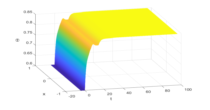 Figure 4. 1: The global asymptotic stability of Θ∗≈0.848 to (4.1) with initial value function 0.6
Limitations & Future Directions
While the paper makes significant strides, it's important to acknowledge its limitations and consider avenues for future development.
One immediate limitation is that the numerical illustration, while compelling, is confined to a specific set of parameters and a one-dimensional spatial domain. While it verifies the theoretical framework for a complex case, it doesn't explore the full parameter space or higher-dimensional scenarios. The "defeat" of baseline models was theoretical (their inability to analyze such problems) rather than a direct numerical comparison of performance or accuracy.
A key open question, explicitly highlighted by the authors, pertains to characterizing the global dynamics of IBVP (1.1) with multiple time-varying delays, particularly under the condition $\sum_{j=1}^m \frac{\beta_j}{\gamma} e^{-a_j \Theta^*} > 1$. The current work focuses on the case where this sum is less than 1 for the zero steady state stability or within a certain range for the positive steady state. Exploring the dynamics when this condition is reversed or falls outside the established bounds would be a crucial next step, potentially revealing more complex behaviors like oscillations or bifurcations.
Looking forward, several diverse perspectives can stimulate further research:
- Generalization to Broader Systems: The authors suggest their analytical framework is adaptable to other delayed diffusive population models, such as the Fisher-KPP equation and Mackey-Glass systems. Future work could explicitly demonstrate this adaptability, applying the methodology to these and other relevant ecological or biological models to establish their stability properties under similar complex delay and parameter conditions.
- Impact of Spatial Heterogeneity and Boundary Conditions: The current work uses a bounded spatial domain with Neumann boundary conditions, implying an isolated habitat. Investigating the effects of different boundary conditions (e.g., Dirichlet for a fixed population at the boundary, or periodic conditions) or more complex, heterogeneous spatial structures could reveal how habitat connectivity and environmental variability influence stability.
- Stochasticity and Environmental Noise: Real-world biological systems are rarely deterministic. Incorporating stochastic perturbations or environmental noise into the delayed diffusive Nicholson's blowflies equation would add another layer of realism. Analyzing how such noise impacts global exponential stability, or if it leads to phenomena like stochastic resonance or noise-induced transitions, would be a fascinating and practically relevant direction.
- Numerical Methods and Computational Efficiency: As the complexity of these models increases, so does the computational cost of their simulation. Developing more efficient and robust numerical schemes specifically tailored for delayed reaction-diffusion equations with time-varying delays and distinct parameters could enable the exploration of larger systems, longer time scales, and higher dimensions, complementing theoretical advancements.
- Biological Interpretation and Predictive Power: Beyond mathematical rigor, a deeper dive into the biological implications of these stability conditions is warranted. How do specific ranges of delay parameters or density-dependent intensities correlate with observed population dynamics in blowflies or other species? Can this model be used to make testable predictions about population outbreaks, extinctions, or the effectiveness of control strategies in pest management? This would bridge the gap between abstract mathematics and applied ecology.
- Critial Parameter Identification: For practical applications, identifying the most influential parameters governing stability is key. Sensitivity analysis could be employed to understand which parameters (e.g., specific delays, birth rates, mortality rates, or density-dependent intensities) have the greatest impact on the global exponential stability of the positive steady state. This could inform experimental design in biology or conservation efforts.
By addressing these points, future research can not only extend the mathematical understanding of delayed diffusive systems but also enhance their utility as predictive tools in various scientific and engineering disciplines.