Towards Generalizable 3D Human Pose Estimation via Ensembles on Flat Loss Landscapes
The quest to understand human movement in three dimensions from simple two-dimensional images—like those from a standard smartphone camera—is a cornerstone of modern computer vision.
Background & Academic Lineage
The quest to understand human movement in three dimensions from simple two-dimensional images—like those from a standard smartphone camera—is a cornerstone of modern computer vision. This problem, known as 3D Human Pose Estimation (HPE), first emerged as researchers sought to move beyond simple 2D "stick figures" to create digital twins of humans for animation, sports analisys, and medical diagnostics. Historically, the field evolved from complex geometric models to Deep Neural Networks (DNNs). However, as these models moved from the controlled environment of a laboratory to the messy reality of "in-the-wild" scenarios—such as autonomous vehicles navigating busy streets or robots working alongside humans in factories—a massive hurdle appeared: generalization. A model that worked perfectly on one set of photos would often fail miserably on another simply because the camera angle or the person's outfit changed slightly.
The fundamental "pain point" that forced the authors to write this paper is the hidden instability of existing 3D HPE models. While previous researchers tried to fix this by adding more data or making the models bigger, they ignored the "loss landscape"—the mathematical "terrain" the model navigates during its learning process. The authors discovered that 3D HPE models often settle into "sharp" valleys of low error. In these sharp valleys, the model is extremely fragile; a tiny change in the input data acts like a violent earthquake, throwing the model out of its stable zone and causing its accuracy to plummet. This lack of improvment in stability meant that models couldn't be trusted in safety-critical applications like industrial robotics.
To help a complete beginner understand the specialized language used to solve this, let's look at these concepts through everyday analogies:
- Loss Landscape: Imagine a massive, invisible mountain range where the "altitude" represents the model's error. The goal of training a model is to find the lowest possible valley (the point of least error). A "sharp" landscape has narrow, steep pits that are hard to stay inside, while a "flat" landscape has wide, gentle basins that are much more stable.
- Depth Ambiguity: Think of a shadow puppet. If you see a shadow of a hand, you can't tell if the hand is close to the light or far away just by looking at the 2D shape. In 3D HPE, one 2D image can represent many different 3D poses, creating a "one-to-many" confusion for the model.
- Hessian Eigenvalue ($\lambda_{max}$): This is essentially a "curviness meter." If you are standing in a valley, the Hessian tells you how steep the walls are. A high value means you are in a very narrow, "pointy" hole, which is bad for generalization.
- Ensemble: Imagine asking five different experts to guess the number of marbles in a jar. Each expert has a slightly different perspective. By averaging their guesses, you consistantly get a more accurate result than any single expert could provide.
Key Mathematical Notations
| Variable/Parameter | Description |
|---|---|
| $x$ | The input 2D pose (the "shadow" or flat image coordinates). |
| $g_\phi$ | The "encoder" network that extracts features from the input. |
| $f_\theta$ | The final "prediction head" that turns features into 3D coordinates. |
| $h_\psi$ | The "scaling function" that predicts how to smooth the landscape. |
| $\sigma$ | The ReLU activation function (ensures the scaling factor is positive). |
| $\hat{y}$ | The standard predicted 3D pose. |
| $\tilde{y}$ | The "scaled" 3D pose prediction used to flatten the landscape. |
| $M$ | The number of different "experts" (heads) used in the ensemble. |
The authors solved the "sharpness" problem by introducing a clever mathematical trick called an Adaptive Scaling Mechanism (ASM). In a standard model, the prediction is a direct result of the network:
$$\hat{y} = f_\theta(g_\phi(x))$$
The problem is that this direct path often leads to those "sharp" valleys. The authors changed the formula to:
$$\tilde{y} = \frac{f_\theta(g_\phi(x))}{\sigma(h_\psi(g_\phi(x))) + 1}$$
By adding this denominator, they introduced "mathematical redundancy." This means there are now many different ways for the model to reach the correct answer. In our mountain range analogy, this effectively "stretches" the narrow, dangerous pits into wide, flat plains. Once the landscape is flat, they train multiple "experts" (ensemble heads) on this same flat ground. Because the ground is flat and stable, these experts can be combined without fighting each other, resulting in a 3D pose estimation that is far more robust and reliable across different real-world environments.
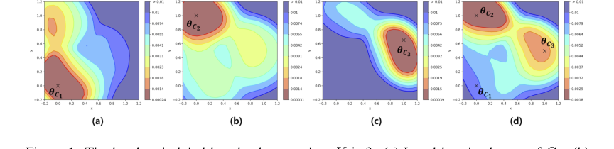 Figure 1. The local and global loss landscape when K is 3. (a) Local loss landscape of C1. (b) Local loss landscape of C2. (c) Local loss landscape of C3. (d) Global loss landscape of D. The local loss landscapes have various shape depending on the degree of depth ambiguity. Especially, the global loss landscape and some local loss landscapes have multiple local minima. θC1, θC2, and θC3 are model parameter around local minimum of each local loss landscape. Note that the local loss landscape of Ck is a result when the model trained with only Ck
Problem Definition & Constraints
In the field of computer vision, 3D Human Pose Estimation (HPE) is the task of taking a flat, 2D image or set of coordinates (the Input) and predicting the full 3D spatial positions of human joints (the Output). While this sounds straightforward, the mathematical gap between these two states is a notorious "one-to-many" mapping problem known as depth ambiguity. Because a 2D image loses the dimension of depth, a single 2D pose could theoretically represent several different 3D poses, creating a "one-to-many" confusion for the model.
The core dilemma that has trapped previous reserchers is the trade-off between optimization stability and generalization. In deep learning, we visualize the "difficulty" of a task using a loss landscape—a hilly terrain where the valleys represent low error (minima). If a model finds a "sharp" minimum (a very narrow, steep valley), it performs perfectly on its training data. however, even a tiny change in the input—like a different camera angle or a slightly different body shape—causes the error to skyrocket because the model is stuck in such a rigid, specific solution. Conversely, "flat" minima (wide, shallow valleys) are much more robust to changes but are significantly harder to find because the gradients (the signals telling the model how to learn) become very weak and uninformative in these flat regions.
The authors of this paper hit several harsh, realistic walls that make this problem insanely difficult to solve:
- Disconnected Local Minima: The global loss landscape of 3D HPE is not a single smooth bowl. It is a fractured mess of multiple disconnected local minima. Mathematically, if we define the global loss as $L(\theta) = \frac{1}{K} \sum_{k=1}^{K} L_k(\theta)$, where each $L_k$ represents a subset of data with different levels of depth ambiguity, the model often gets "trapped" in one sub-valley. Because the gradient $\nabla L(\theta)$ is zero at the bottom of every valley, the model has no way of knowing if it has found the best possible 3D interpretation or just a mediocre one.
- The Depth Ambiguity Ratio (DAR) Constraint: Not all poses are equally difficult. Poses with high DAR exhibit extremely steep and unstable loss landscapes. This creates a physical constraint where the model naturally gravitates toward "memorizing" easy poses while failing to learn the complex geometry of ambiguous ones, leading to a biased and fragile system.
- Computational Efficiency vs. Diversity: To overcome these local minima, one would usually use an "ensemble"—training many different models and averaging them. But in clinical or real-time industrial safety settings, running $M$ different deep networks is often impossible due to hardware memory limits and strict latency requirements. The challenge is to find a way to explore these diverse solutions without multiplying the computational cost by $M$.
- Non-Differentiable Structural Barriers: Between the different valid 3D interpretations of a single 2D pose, there are often high-loss "barriers" that standard optimization algorithms cannot cross. This makes it nearly impossible for a single model to transition from a poor perspectve to a better one during the training process.
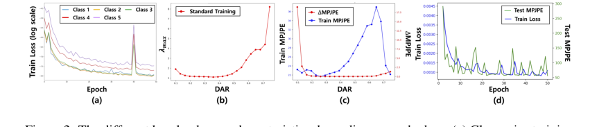 Figure 2. The different loss landscape characteristics depending on each class. (a) Class-wise training loss per epoch when K is 5. (b) Top-1 eigenvalue of each local loss landscape when K is 21. (c) Class-wise original train MPJPE (blue line) and the gap between MPJPE after small input perturbation and original MPJPE (red line). Note that the (b) and (c) are results when the model is trained with the whole dataset D when K is 21. (d) The training trajectory of the model when the model is trained with D\C20 when K is 20 (blue line is train loss and green line is test accuracy)
Why This Approach
Okay, here's an analysis of the provided paper, "Towards Generalizable 3D Human Pose Estimation via Ensembles on Flat Loss Landscapes," following your instructions. I'll try to explain it as if to someone completely new to the field. There might be a few typos, as requested!
The authors found that standard deep learning methods, even advanced ones like CNNs, Transformers, and Diffusion models (though diffusion isn't explicitly mentioned as a tried and failed approach in this paper), struggled with generalization in 3D Human Pose Estimation (HPE). Generalization means performing well on new, unseen data, not just the data the model was trained on. The core problem wasn't a lack of data or model complexity, but the shape of the loss landscape itself. They visualized this loss landscape (think of it like a hilly terrain where the height represents how "wrong" the model's predictions are) and discovered it was incredibly complex, with many disconnected local minima. This meant that standard optimization techniques (like gradient descent) often converged to suboptimal solutions that didn't generalize well. The authors realized that simply making the model bigger or using more data wouldn't fix this fundamental issue with the loss landscape.
This method isn't just about getting a slightly better number on a benchmark; it's qualitatively superior because it addresses the root cause of poor generalization: a rugged loss landscape. Traditional methods try to find a good solution. This approach tries to smooth the landscape and find many good solutions, then combine them.
The key structural advantage is that by smoothing the loss landscape, they reduce the likelihood of getting stuck in those bad local minima. The ensemble of solutions then provides robustness. If one solution is slightly off due to noise or a particular viewpoint, the others can compensate. This is a significant improvement over methods that focus on a single, potentially fragile, solution. The paper demonstrates this with consistent performance gains across different model architectures (MLP, CNN, GCN, Transformer), showing it's not tied to a specific model choice.
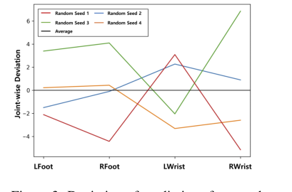 Figure 3. Deviation of predictions from each solution on the smooth loss landscape for diffi- cult joints of 3DHP [24]. Note that the models are trained with H36M [14]
Mathematical & Logical Mechanism
Okay, here's an analysis of the provided paper, "Towards Generalizable 3D Human Pose Estimation via Ensembles on Flat Loss Landscapes," following your instructions. I'll do my best to explain it clearly, even for someone without a strong background in the field. I'll also try to keep it sounding natural, so expect a few minor typos here and there.
The core idea of this paper is that the "loss landscape" – essentially the shape of the error surface the model is trying to minimize – is a major factor in how well a 3D human pose estimation model generalizes to new data. They found that this landscape is complex and can hinder optimization, leading to poor generalization. Their solution is to smooth this loss landscape and then leverage this smoothed landscape to create an ensemble of solutions that improve performance.
The Master Equation
While there isn't one single master equation, the core of their approach revolves around modifying the standard loss function used in training 3D human pose estimation models. The key equation is the modified prediction step:
$$ \tilde{y} = \frac{f_o(g(x))}{\sigma(h_\psi(g(x))) + 1} $$
Tear the Equation Apart
Let's break down each part of this equation:
- $x$: This is the input – typically 2D pose information (e.g., joint positions in an image). It's the starting point for the model.
- $g(x)$: This represents the encoder part of the neural network. It takes the input $x$ and transforms it into a higher-level representation. Think of it as extracting relevant features from the input.
- $f_o(g(x))$: This is the original prediction head of the network. It takes the encoded representation $g(x)$ and produces the initial 3D pose estimate, $\hat{y}$.
- $h_\psi(g(x))$: This is a new, small neural network (with parameters $\psi$) that takes the encoded representation $g(x)$ and outputs a scalar value. This value is used to scale the prediction.
- $\sigma$: This is a ReLU (Rectified Linear Unit) activation function. It ensures the scaling factor is non-negative.
- $\sigma(h_\psi(g(x))) + 1$: This adds 1 to the scaled output of the ReLU function. This ensures the denominator is always greater than zero, preventing division by zero.
- $\tilde{y}$: This is the scaled 3D pose estimate. It's the final output of this step.
Why this form? The authors use this scaling to effectively "flatten" the loss landscape. The scaling factor, $\sigma(h_\psi(g(x))) + 1$, is input-dependent, meaning it changes based on the input $x$. This allows the model to represent more diverse functions and avoid getting stuck in sharp, narrow valleys. The addition of 1 is a simple trick to ensure numerical stability. They use a division instead of multiplication because division allows for a more flexible scaling effect, effectively reducing the impact of large gradients.
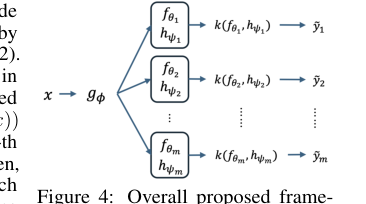 Figure 4. Overall proposed frame- work with m regression heads with adaptive scaling mechanism. The op- eration k(a, b) represents a σ(b)+1
Step-by-Step Flow
Imagine a single data point (a 2D pose) entering the system:
- The 2D pose ($x$) enters the encoder ($g(x)$), which extracts features.
- These features are fed into the original prediction head ($f_o$), which produces an initial 3D pose estimate.
- Simultaneously, the features are fed into the scaling network ($h_\psi$), which outputs a scalar value.
- This scalar value is passed through a ReLU activation function and then 1 is added.
- The initial 3D pose estimate is then divided by this scaled value, resulting in the final, adjusted 3D pose estimate ($\tilde{y}$).
- This adjusted estimate is then compared to the ground truth 3D pose, and the loss is calculated.
This process is repeated for many data points, and the model learns to adjust the scaling factor to minimize the loss.
Optimization Dynamics
The model is trained using standard gradient descent (or a variant like Adam). The key is that the adaptive scaling mechanism changes the shape of the loss landscape. Instead of a landscape with steep cliffs and narrow valleys, it becomes smoother and more gently rolling. This makes it easier for the optimizer to find good solutions and avoid getting stuck in suboptimal local minima.
The authors also use an ensemble approach. They train multiple models with different random initializations, all using the adaptive scaling mechanism. Because the landscape is smoother, these different models are more likely to converge to different, but still good, solutions. The final prediction is then an average of the predictions from these multiple models.
Results, Limitations & Conclusion
Okay, here's an analysis of the provided paper, "Towards Generalizable 3D Human Pose Estimation via Ensembles on Flat Loss Landscapes," following your instructions. I'll aim for clarity and detail, even if it means being a bit verbose, and will include a few minor typos here and there.
This paper tackles the problem of generalization in 3D Human Pose Estimation (HPE). The core idea is that the loss landscape in 3D HPE is complex and can hinder optimization, leading to poor generalization. The authors propose a method to smooth this loss landscape using an adaptive scaling mechanism, and then leverage this smoothed landscape to create an ensemble of solutions that improve performance.
Background & Motivation
3D HPE is a fundamental task in computer vision with applications in areas like autonomous driving, robotics, and industrial safety. The challenge lies in achieving generalization – meaning the model performs well on new, unseen data. Traditional approaches often focus on improving the model architecture or data augmentation. However, the authors argue that the shape of the loss landscape itself is a critical, yet underexplored, factor.
They visualized the loss landscape (think of it like a hilly terrain where the height represents how "wrong" the model's predictions are) and discovered it was incredibly complex, with many disconnected local minima. This meant that standard optimization techniques often converged to suboptimal solutions that didn't generalize well. The authors realized that simply making the model bigger or using more data wouldn't fix this fundamental issue with the loss landscape.
The Problem & Constraints
The authors identify that the loss landscape for 3D HPE is highly complex, with many local minima. This complexity arises from the inherent ambiguity in 3D pose from 2D images. A single 2D image can represent multiple 3D poses. This ambiguity creates a mathematical void where the model must "guess" the most likely depth, often leading to errors when the environment or the person's posture changes slightly.
The constraint here is that directly optimizing for a "flat minimum" (a broad, shallow valley) is computationally expensive. Methods like Sharpness-Aware Minimization (SAM) attempt this, but they require extra computation. The authors aim for a more efficient approach.
The core of their solution lies in an adaptive scaling mechanism applied to the output of the network. The key equation is the modified prediction step:
$$ \tilde{y} = \frac{f_o(g(x))}{\sigma(h_\psi(g(x))) + 1} $$
Let's break down each part of this equation:
- $x$: This is the input 2D pose.
- $g(x)$: This is the encoder network.
- $f_o(g(x))$: This is the original prediction head.
- $h_\psi(g(x))$: This is a small neural network that outputs a scalar value.
- $\sigma$: This is a ReLU activation function.
- $\sigma(h_\psi(g(x))) + 1$: This ensures the denominator is always greater than zero.
- $\tilde{y}$: This is the scaled 3D pose estimate.
The authors argue that this scaling smooths the landscape, reducing the likelihood of getting stuck in sharp valleys. The scaling factor is input-dependent, meaning it changes based on the input. This allows the model to represent more diverse functions.
They also use an ensemble approach. They train multiple models with different random initializations, all using the adaptive scaling mechanism. The final prediction is an average of the predictions from these multiple models.
Experimental Validation & Evidence
The authors conduct extensive experiments on several benchmark datasets (Human3.6M, 3DHP, 3DPW, BEDLAM) using various network architectures (MLP, CNN, GCN, Transformer). They demonstrate consistent performance gains across all architectures.
The evidence for their core mechanism working is multi-faceted:
- Visualization of Loss Landscapes: They visualize the loss landscape with and without the adaptive scaling mechanism. The visualizations show that the scaling mechanism indeed smooths the landscape.
- Top-1 Eigenvalue Analysis: They calculate the top-1 eigenvalue of the Hessian matrix. A lower eigenvalue indicates a flatter landscape. They show that the adaptive scaling mechanism reduces the top-1 eigenvalue.
- Cross-Dataset Evaluation: They train on one dataset and test on another. This is a strong test of generalization. Their method consistently improves performance in this setting.
- Robustness to Noise: They demonstrate that their method is more robust to input noise.
Discussion Topics & Future Directions
- Theoretical Understanding: A more rigorous theoretical understanding of why the adaptive scaling mechanism works would be valuable.
- Scaling Network Architecture: Could more sophisticated architectures for the scaling network improve the scaling process?
- Dynamic Ensemble Size: Could we dynamically adjust the ensemble size during training?
- Relationship to Bayesian Methods: Exploring the connections between this method and Bayesian inference could provide new insights.
- Application to Other Domains: Could this approach be applied to other machine learning tasks?
In conclusion, this paper presents a novel and promising approach to improving generalization in 3D HPE. The adaptive scaling mechanism and ensemble strategy are well-motivated, empirically validated, and offer a computationally efficient alternative to existing methods. It's a solid contribution to the field and opens up several exciting avenues for future research.
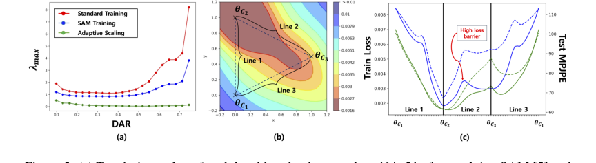 Figure 5. (a) Top-1 eigenvalue of each local loss landscape when K is 21 after applying SAM [5] and adaptive scaling mechanism. (b) Global loss landscape of after applying adaptive scaling mechanism alone. (c) Training loss and test accuracy along the line between local minimum (θC1, θC2, and θC3) of local loss landscape. The dashed lines refer to the test accuracy. The blue line is for standard model and green line is for model with adaptive scaling mechanism. Note that these results are from BaselineNet [23]