SOO-Bench: Benchmarks for Evaluating the Stability of Offline Black-Box Optimization
The problem of Offline Black-Box Optimization (BBO) emerged from the practical necessity of optimizing complex systems where direct, real-time evaluation of the objective function is either too dangerous,...
Background & Academic Lineage
The Origin & Academic Lineage
The problem of Offline Black-Box Optimization (BBO) emerged from the practical necessity of optimizing complex systems where direct, real-time evaluation of the objective function is either too dangerous, prohibitively expensive, or physically impossible. Historically, BBO methods relied on "active sampling"—iteratively querying the system to learn its behavior. However, in domains like drug discovery (e.g., designing molecular structures) or hardware engineering (e.g., mechanical structure parameters), we cannot simply "test" a new design on the fly. Instead, researchers are forced to rely on a static, pre-existing "offline" dataset of historical experiments.
The fundamental "pain point" that motivated this paper is the narrow distribution of these offline datasets. Because historical data is often collected based on subjective experimenter bias or specific, limited strategies, it fails to cover the entire solution space. Previous algorithms, when trained on such narrow data, often suffer from the "out-of-distribution" (OOD) problem: they become overconfident in regions where they have no data, leading to performance degradation during optimization. Furthermore, existing benchmarks like Design-Bench were primarily designed to provide tasks and datasets but lacked the capability to evaluate the stability of an algorithm—its ability to consistently improve upon the offline dataset without being misled by the narrow data distribution.
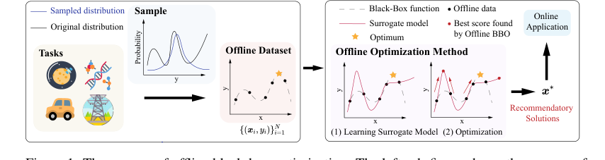 Figure 1. The process of offline black-box optimization. The left sub-figure shows the process of collecting offline data from a real black-box objective function. The right sub-figure shows the process of an offline optimization algorithm finding satisfied solutions for online application
Intuitive Domain Terms
- Black-Box Optimization (BBO): Imagine trying to find the perfect recipe for a cake, but you aren't allowed to taste the batter or see the ingredients list. You can only bake a cake and have a judge give you a score. BBO is the mathematical process of finding the best "recipe" (input) based only on these scores, without knowing the underlying "chemistry" (the function) of the cake.
- Surrogate Model: Since evaluating the real "black-box" is expensive, we build a "digital twin" or a simplified mathematical approximation of it. We train this model on our historical data so we can "test" millions of potential solutions on the model instead of the real, costly system.
- Narrow Distribution: Think of this as a student who has only ever studied questions from Chapter 1 of a textbook. If you give them a test covering the whole book, they will likely fail because they have no experience with the material in the other chapters. In optimization, if our historical data only covers a small, specific area, the model won't know how to behave when it wanders into "unseen" territory.
- Out-of-Distribution (OOD): This refers to the "unseen territory" mentioned above. It is the region of the solution space that is not represented in the historical data. Algorithms often "hallucinate" or make wild, incorrect guesses about how good a solution is in these regions because they have no data to ground their predictions.
Notation Table
| Notation | Description |
|---|---|
| $f: \mathcal{X} \to \mathbb{R}$ | The unknown black-box objective function. |
| $\mathcal{X} \subseteq \mathbb{R}^d$ | The $d$-dimensional solution space. |
| $\mathcal{D} = \{x_i, y_i\}_{i=1}^N$ | The static offline dataset containing $N$ solutions and their values. |
| $\hat{f}_\theta(x)$ | The surrogate model with parameters $\theta$ trained on $\mathcal{D}$. |
| $x^{(t)}$ | The solution at optimization step $t$. |
| $\eta$ | The learning rate (step size) for the optimization process. |
| $T$ | The total number of optimization steps. |
| $x_{\text{app}} = x^{(T)}$ | The final solution output for online application. |
| $SO$ | The Stability-Optimality indicator. |
| $OI(t)$ | The Optimality Indicator at step $t$. |
| $SI(t)$ | The Stability Indicator at step $t$. |
The authors address the problem of finding an optimal solution $x^*$ by maximizing $f(x)$ without direct interaction. The core challenge is that the surrogate model $\hat{f}_{\theta^*}(x)$ is only reliable near the data in $\mathcal{D}$. The optimization process typically follows gradient ascent:
$$x^{(t+1)} \leftarrow x^{(t)} + \eta \nabla_x \hat{f}_{\theta^*}(x)|_{x=x^{(t)}}$$
The "pain point" is that as $t$ increases, $x^{(t)}$ may drift into OOD regions where $\hat{f}_{\theta^*}(x)$ is inaccurate, causing the performance to collapse.
To solve this, the authors propose the Stability-Optimality (SO) indicator to quantify how well an algorithm balances finding the global optimum (Optimality) with staying within a reliable region (Stability). The SO is defined as:
$$SO = \frac{2 \cdot OI(t) \cdot SI(t)}{SI(t) + OI(t)}$$
where $OI(t) = \frac{S}{S_1}$ and $SI(t) = \frac{S}{S_2}$. Here, $S$ is the cumulative sum of the algorithm's performance, $S_1$ represents the "ideal" performance based on the offline dataset's best solution, and $S_2$ represents the performance relative to the best solution the algorithm has found so far. By maximizing $SO$, the algorithm is forced to not only find good solutions but to maintain them, preventing the performance degradation that plagues previous models. The authors also introduce a weighted version, $SO_\omega$, to allow users to prioritize either stability or optimality depending on their specific needs.
Problem Definition & Constraints
Core Problem Formulation & The Dilemma
In standard black-box optimization (BBO), an algorithm actively samples solutions and evaluates their objective function values to find an optimum. However, in many critical real-world domains—such as drug discovery or hardware mechanical design—evaluating a new solution is often dangerous, prohibitively expensive, or physically impossible. This necessitates Offline Black-Box Optimization, where the algorithm must rely solely on a static, pre-existing dataset $\mathcal{D} = \{x_i, y_i\}_{i=1}^N$ to learn a surrogate model $\hat{f}_\theta(x)$ and subsequently identify an optimal solution $x_{app}$.
The Dilemma:
The fundamental challenge is the narrow distribution of the offline dataset. Because data collection is often biased by human expertise or specific experimental constraints, the dataset rarely covers the entire solution space. Consequently, the surrogate model $\hat{f}_\theta(x)$ becomes highly inaccurate in "out-of-distribution" (OOD) regions. If an algorithm attempts to find an optimum far from the known data, the surrogate model often overestimates the objective value, leading to severe performance degradation during the optimization process.
The Constraints:
Researchers face a "stability vs. optimality" trade-off. An algorithm that aggressively pursues the global optimum may easily fall into OOD traps, while one that is too conservative may fail to improve upon the best solution already present in the dataset. The authors identify several harsh, realistic walls:
1. Lack of Ground Truth: In many real-world tasks, the true global optimum is unknown, making it difficult to measure how well an algorithm performs.
2. Data Sparsity: The limited size and uneven distribution of historical data make it difficult to train a reliable surrogate model.
3. Stability Evaluation: There has been no standardized, quantitative metric to evaluate whether an algorithm can consistently surpass the offline dataset without suffering from performance collapse as it explores unknown regions.
The authors bridge the gap between current state (limited offline data) and goal state (stable, high-quality online solutions) by introducing SOO-Bench and a novel Stability-Optimality (SO) indicator.
The problem is formulated as finding $x_{app}$ by maximizing the surrogate model $\hat{f}_\theta(x)$ via iterative gradient ascent:
$$x^{(t+1)} \leftarrow x^{(t)} + \eta \nabla_x \hat{f}_{\theta^*}(x)|_{x=x^{(t)}}, \quad t = 1, 2, \dots, T$$
where $x_{app} = x^{(T)}$.
To quantify stability, the authors define the Stability-Optimality (SO) indicator, which balances two components:
1. Optimality Indicator (OI): Measures the ratio of the area under the algorithm's evaluation curve to the area under the offline optimal solution curve.
$$OI(t) = \frac{S}{S_1}, \quad S = \sum_{t=1}^T f(x_t), \quad S_1 = T \cdot f(x^*_{OFF})$$
2. Stability Indicator (SI): Measures how closely the algorithm's performance aligns with the best solution it has found so far, effectively penalizing fluctuations.
$$SI(t) = \frac{S}{S_2}, \quad S_2 = T \cdot \max_t f(x_t)$$
The final SO score is the harmonic mean of these two, ensuring that a high score requires both high performance (optimality) and consistent behavior (stability):
$$SO = \frac{2 \cdot OI(t) \cdot SI(t)}{SI(t) + OI(t)}$$
By providing customizable datasets (adjusting the removal of top/bottom solutions) and this SO indicator, the authors enable researchers to systematically test how algorithms handle OOD regions, effectively forcing them to prove their robustness against the "narrow distribution" trap.
Why This Approach
The core challenge in offline black-box optimization (BBO) is the "narrow distribution" of historical data. Traditional methods, such as standard CNNs or basic Transformers, are designed to learn from broad, representative datasets. However, in real-world scenarios like drug discovery or satellite trajectory design, the available data is often collected through biased or limited strategies, meaning it does not cover the entire solution space.
Why this approach?
The authors identified that traditional methods fail because they are "misled" by this narrow data. When a surrogate model is trained on a narrow dataset, it often overestimates the quality of solutions in regions where it has no data (the out-of-distribution or OOD regions). This leads to a catastrophic degradation in performance during the optimization process.
- Comparative Superiority: Unlike previous benchmarks like Design-Bench, which used fixed, artificially constructed narrow distributions, SOO-Bench allows for the customization of these distributions. This structural advantage is critical because it enables researchers to stress-test algorithms against varying levels of "narrowness," effectively simulating the unpredictable nature of real-world data collection.
- The "Marriage" of Requirements: The paper introduces the Stability-Optimality (SO) indicator. This is the "marriage" between the harsh requirement of needing to surpass the offline dataset and the constraint of not being misled by OOD regions. By mathematically combining an Optimality Indicator (OI) and a Stability Indicator (SI), the model forces algorithms to prove they can not only find a good solution but also maintain that performance throughout the optimization steps.
- Why other methods fail: The authors reject simple, non-conservative approaches because they lack a mechanism to penalize the model for exploring high-risk, OOD regions. Methods like ARCOO are highlighted because they explicitly incorporate a "risk suppression factor" to control the step size during gradient ascent, preventing the model from wandering into dangerous, unverified territory.
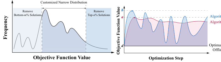 Figure 2. The illustrations of narrow data distribution issue consider and address in SOO-Bench and the motivation of stability indicator
The problem is defined as finding an optimal solution $x^*$ that maximizes a black-box function $f(x)$, where $f$ is approximated by a surrogate model $\hat{f}_\theta(x)$ trained on a static dataset $\mathcal{D} = \{x_i, y_i\}_{i=1}^N$. The optimization process typically follows:
$$x^{(t+1)} \leftarrow x^{(t)} + \eta \nabla_x \hat{f}_{\theta^*}(x)|_{x=x^{(t)}}$$
The authors realized that if $T$ (the number of steps) is too large, the algorithm drifts into OOD regions. To solve this, they proposed the SO indicator:
$$SO = \frac{2 \cdot OI(t) \cdot SI(t)}{SI(t) + OI(t)}$$
where $OI(t) = \frac{S}{S_1}$ and $SI(t) = \frac{S}{S_2}$. Here, $S$ is the cumulative sum of the evaluation curve, $S_1$ represents the product of the offline optimal value and total steps, and $S_2$ represents the product of the algorithm's best-found value and total steps. This model effectively penalizes algorithms that show high variance or "unstable" performance, ensuring that the algorithm's trajectory remains robust even when the surrogate model is imperfect.
The approach is fundamentally superior because it moves the field from "finding the best point" to "finding the best point while staying safe." It is a shift from pure performance to reliable performance, which is the only viable path for high-stakes engineering tasks where a bad guess could be perilous.
Mathematical & Logical Mechanism
The Master Equation
The core mechanism of the paper is the Stability-Optimality (SO) indicator, which evaluates how well an offline optimization algorithm performs relative to the offline dataset's best solution while maintaining stability throughout the optimization process. The primary equation is:
$$SO = \frac{2 \cdot OI(t) \cdot SI(t)}{SI(t) + OI(t)}$$
Where the components are defined as:
$$OI(t) = \frac{S}{S_1}, \quad SI(t) = \frac{S}{S_2}$$
Tearing the Equation Apart
- $S = \sum_{t=1}^{T} f(x_t)$: This is the cumulative sum of the objective function values across all optimization steps $T$. It represents the total "performance footprint" of the algorithm.
- $S_1 = T \cdot f(x^*_{\text{OFF}})$: This is the baseline reference. It represents the performance if the algorithm had consistently achieved the best value found in the offline dataset ($f(x^*_{\text{OFF}})$) for every single step $T$.
- $S_2 = T \cdot \max_t f(x_t)$: This is the peak performance reference. It represents the performance if the algorithm had consistently achieved its own best-found value ($\max_t f(x_t)$) for every step $T$.
- $OI(t)$ (Optimality Indicator): This ratio measures the algorithm's performance relative to the offline dataset's best. If $OI > 1$, the algorithm is successfully surpassing the offline data.
- $SI(t)$ (Stability Indicator): This ratio measures how closely the algorithm's performance aligns with its own peak. A value near 1 indicates high stability (minimal fluctuation), while a low value suggests the algorithm is "jittery" or prone to performance degradation.
- The Harmonic Mean ($2 \cdot \frac{OI \cdot SI}{SI + OI}$): The authors use the harmonic mean instead of a simple arithmetic average to ensure that the SO indicator is sensitive to both components. If either $OI$ or $SI$ is very low, the harmonic mean pulls the total score down significantly, effectively penalizing algorithms that are either unstable or fail to surpass the offline dataset.
Step-by-Step Flow
The lifecycle of an abstract data point in this system follows this assembly line:
- Initialization: The algorithm starts with an offline dataset $\mathcal{D}$. It trains a surrogate model $\hat{f}_\theta(x)$ to approximate the black-box function.
- Optimization: The algorithm performs gradient ascent for $T$ steps to find a new solution $x_{\text{app}}$.
- Evaluation: At each step $t$, the algorithm produces a solution $x_t$. The system calculates the objective value $f(x_t)$.
- Aggregation: These values are summed into $S$. Simultaneously, the system tracks the best offline value ($f(x^*_{\text{OFF}})$) and the algorithm's own best value ($\max_t f(x_t)$).
- Indicator Calculation: The system computes $OI(t)$ and $SI(t)$ to quantify how much better the algorithm is than the offline data and how stable its trajectory is.
- Final Score: The SO indicator combines these into a single metric, providing a quantitative "grade" for the algorithm's stability and optimality.
Optimization Dynamics
The mechanism learns by iteratively updating the surrogate model $\hat{f}_\theta(x)$ using supervised learning on the offline dataset $\mathcal{D}$. The loss function is:
$$\theta^* \leftarrow \arg \min_\theta \sum_{i=1}^N (\hat{f}_\theta(x_i) - y_i)^2$$
The optimization process then uses gradient ascent to navigate the surrogate model's landscape:
$$x^{(t+1)} \leftarrow x^{(t)} + \eta \nabla_x \hat{f}_{\theta^*}(x)|_{x=x^t}$$
The "learning" here is essentially the surrogate model's ability to generalize from the narrow distribution of the offline data to the broader solution space. The stability is maintained by the risk suppression factors (like in the ARCOO algorithm) which act as a "governor" on the gradient ascent, preventing the model from overestimating values in out-of-distribution (OOD) regions where it lacks data. This prevents the model from being "misled" by its own overconfidence, which is a common failure mode in offline BBO.
Results, Limitations & Conclusion
Black-Box Optimization (BBO) is a method for finding the optimal input $x^*$ that maximizes an objective function $f(x)$ without knowing the explicit mathematical form of $f$. In traditional BBO, an algorithm can actively sample points and evaluate them. However, in many real-world scenarios (e.g., drug discovery, mechanical design), evaluating $f(x)$ is too expensive or dangerous. This leads to Offline BBO, where the algorithm must learn a surrogate model $\hat{f}_\theta(x)$ using only a static, pre-collected dataset $\mathcal{D} = \{x_i, y_i\}_{i=1}^N$.
The core challenge here is the narrow distribution of the offline dataset. Because the data is often collected based on human bias or specific experimental constraints, it does not cover the entire solution space. A surrogate model trained on this data often becomes "misled" when it tries to predict values in regions far from the training data (Out-of-Distribution or OOD regions), leading to poor optimization performance.
The authors argue that existing benchmarks (like Design-Bench) focus primarily on optimality—finding the best possible solution. However, in high-stakes engineering, stability is just as critical. Stability is defined as the algorithm's ability to consistently find solutions that surpass the best known solution in the offline dataset without being misled by the narrow data distribution. The authors identify that current benchmarks lack a quantitative way to measure this stability.
The paper introduces the Stability-Optimality (SO) indicator to quantify how well an algorithm performs throughout the optimization process. For a total of $T$ optimization steps, let $f(x_t)$ be the evaluation of the solution at step $t$. The indicator is defined as:
$$SO = \frac{2 \cdot OI(t) \cdot SI(t)}{SI(t) + OI(t)}$$
Where:
* Optimality Indicator (OI): $OI(t) = \frac{S}{S_1}$, where $S = \sum_{t=1}^T f(x_t)$ and $S_1 = T \cdot f(x^*_{OFF})$. This measures the ratio of the area under the algorithm's performance curve to the area under the baseline (the best solution in the offline dataset).
* Stability Indicator (SI): $SI(t) = \frac{S}{S_2}$, where $S_2 = T \cdot \max_t f(x_t)$. This measures how closely the algorithm's performance aligns with the best solution it has found so far.
The authors also propose a weighted version, $SO_\omega$, which allows users to prioritize either optimality or stability during different phases of the optimization process.
Experimental Proof
The authors architected SOO-Bench to "ruthlessly" test algorithms by:
1. Customizing Data Difficulty: They created datasets by removing the top $n\%$ (making it harder to find high-quality solutions) and bottom $m\%$ (increasing sparsity) of the data.
2. Diverse Tasks: They included real-world tasks from satellite trajectory optimization (GTOPX), industrial design (CEC), and DNA sequence design (PROTEIN).
3. Baseline Comparison: They tested state-of-the-art (SOTA) algorithms, including ARCOO, Tri-mentoring, and TTDDEA, against classical baselines like BO-qEI and CMA-ES.
The "victims" (baseline models) were often shown to be highly sensitive to OOD regions. The definitive evidence provided is that while some algorithms (like ARCOO) maintain stable performance by using an energy-based model to suppress risk, others (like DE-PF and DE-SPF) show poor SO values, indicating they frequently fall into infeasible regions or stagnate.
Discussion Topics for Future Development
- Dynamic Weighting: The authors use a linearly decreasing weight function $\omega(t)$ for $SO_\omega$. Could we develop an adaptive weighting mechanism that senses the surrogate model's uncertainty and shifts priority between optimality and stability in real-time?
- Beyond OOD: How can we extend SOO-Bench to handle "concept drift" in offline datasets, where the underlying physics or constraints of the problem might change over time?
- Constraint Handling: The paper notes that current methods struggle with strict constraints. Future work could explore how to incorporate "soft" constraint satisfaction into the surrogate model training to prevent the algorithm from becoming too conservative and stagnating.
Overall, this paper provides a much-needed, rigorous framework for a field that has been somewhat "wild west" in its evaluation metrics.
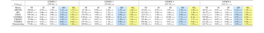 Table 2. Overall results for GTOPX unconstrained tasks with 128 solutions and 100th percentile evaluations are averaged over eight runs. f(x∗ OFF) represents the optimal objective function value in the offline dataset. FS (i.e., final score) refers to the function value found by an offline optimization algorithm at t = 50 during the optimization process, which consists of a total of T = 150 optimization steps. In this case, 25% of the values are missing near the worst value and another 25% near the optimal value
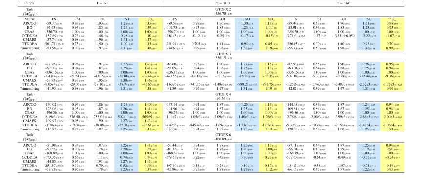 Table 5. Overall results for GTOPX unconstrained tasks with 128 solutions and 100th percentile evaluations are averaged over eight runs. f(x∗ OFF) represents the optimal objective function value in the offline dataset. FS (i.e., final score) refers to the function value found by an offline optimization algorithm at the final step of specific optimization steps (i.e., t = 50, 100, 150). The symbol "-“ means that the algorithm cannot complete the corresponding task within 24 hours. In this case, 0% of the values are missing near the worst value and another 50% near the optimal value
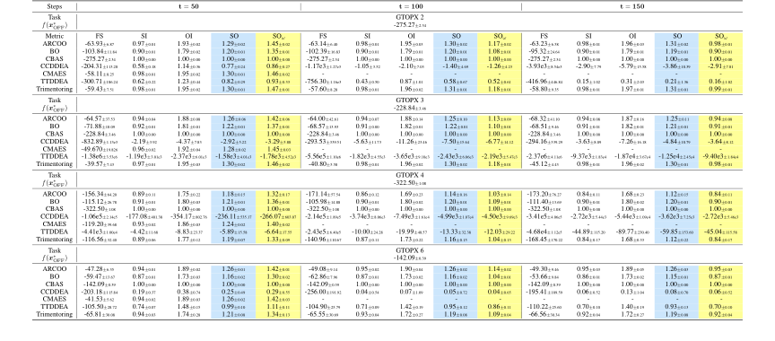 Table 6. Overall results for GTOPX unconstrained tasks with 128 solutions and 100th percentile evaluations. In this case, 0% of the values are missing near the worst value and another 40% near the optimal value. Details are the same as Table 5
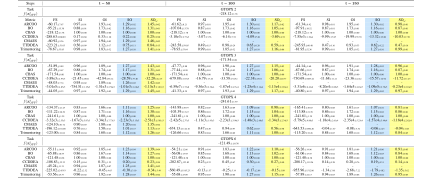 Table 7. Overall results for GTOPX unconstrained tasks with 128 solutions and 100th percentile evaluations. In this case, 0% of the values are missing near the worst value and another 30% near the optimal value. Details are the same as Table 5