VesselSDF: Distance Field Priors for Vascular Network Reconstruction
ISOM uses this paper to study how distance fields can preserve vascular topology when local segmentation confidence is not enough.
Background & Academic Lineage
The Origin & Academic Lineage
The problem of accurately reconstructing vascular networks from medical imaging data, particulary from sparse CT scan slices, has long been a fundamental challenge in clinical diagnostics and surgical planning. This issue first emerged and gained prominence as medical imaging technologies, like Computed Tomography (CT), became indispensable for diagnosing conditions ranging from coronary artery disease to tumor assessment. Early approaches to segmenting these intricate, tree-like structures often relied on traditional image processing techniques. However, as the demand for more precise 3D models of vessels grew for surgical navigation, blood flow dynamics analysis, and early detection of abnormalities, the limitations of these methods became increasingly apparent. The advent of deep learning brought significant advancements to medical image segmentation, but even these sophisticated models struggled with the unique characteristics of vascular networks.
The fundamental "pain points" that forced the authors to develop VesselSDF stem from three critical limitations of previous approaches:
- Jagged Surface Artifacts: Traditional binary voxel classification methods represent vessels as discrete 3D cubes. This discrete nature often leads to jagged, blocky surfaces in the reconstructed vessels, which is especially problematic for thin vessels where the surface-to-volume ratio is high. This lack of smoothness makes the models less accurate for clinical applications.
- Anisotropic Distortions and Fragmentation: Medical CT scans often have a much higher resolution within each slice (in-plane, $\Delta x, \Delta y$) compared to the spacing between slices (slice thickness, $\Delta z$). This significant difference creates anisotropic distortions, causing vessels to appear fragmented or disconnected, especially at branching points or where they change direction rapidly.
- Floating Artifacts in SDFs: While Signed Distance Fields (SDFs) offer a promising way to represent continuous surfaces, existing SDF-based methods themselves often generate "floating artifacts"—small, disconnected surface fragments that appear in the reconstruction but do not correspond to actual vessel structures, thereby degrading the overall quality and reliability of the 3D model.
Intuitive Domain Terms
- Signed Distance Field (SDF): Imagine you have a 3D map of a city, and you want to know how far every point in the city is from the nearest river. An SDF is like that map, but for a vessel. For any point in space, it tells you the shortest distance to the vessel's surface. If the point is inside the vessel, the distance is negative; if it's outside, it's positive; and if it's exactly on the surface, the distance is zero. This continuous representation helps capture smooth shapes.
- Binary Voxel Classification: Think of a 3D image as being made up of tiny LEGO bricks (voxels). Binary voxel classification is like deciding for each individual LEGO brick whether it's part of a vessel (you color it red) or not part of a vessel (you leave it clear). It's a simple "yes" or "no" decision for each tiny cube, which can lead to blocky or fragmented results.
- Sparse CT Scan Slices: Imagine trying to understand the full 3D shape of a complex tree by only looking at a few very thin, widely spaced cross-sections of its trunk and branches. A sparse CT scan is similar: you get limited "slices" of the body, and there are significant gaps between them. Reconstructing continuous structures like blood vessels from these few, distant slices is a major challenge.
- Structural Continuity / Geometic Fidelity: This refers to how well a reconstructed vessel maintains its natural, unbroken flow and accurate shape. If a vessel is supposed to be a continuous tube, "structural continuity" means it doesn't have gaps or breaks. "Geometric fidelity" means its curves, branches, and diameters accurately match the real vessel, rather than being jagged, distorted, or simplified.
- Floating Artifacts: Picture a sculptor trying to carve a detailed statue, but accidentally leaving tiny, unwanted chips of stone floating around the main sculpture. In 3D vessel reconstruction, floating artifacts are small, disconnected pieces of geometry that appear in the final model but don't belong to the actual vessel network. They are spurious elements that degrade the quality and realism of the reconstruction.
Notation Table
| Notation | Description |
|---|---|
| $V$ | Input volumetric CT scan |
| $D, H, W$ | Dimensions of the CT scan (Depth, Height, Width) |
| $\mathbf{x}$ | A 3D spatial coordinate in $\mathbb{R}^3$ |
| $f_{SDF}(\mathbf{x}; \theta_r)$ | Predicted Signed Distance Field (SDF) at $\mathbf{x}$, parameterized by $\theta_r$ |
| $S$ | The vessel surface, defined as the zero-level set of $f_{SDF}$ |
| $f_o(\mathbf{x}; \theta_o)$ | Predicted binary occupancy probability at $\mathbf{x}$, parameterized by $\theta_o$ |
| $f^*_{SDF}(\mathbf{x})$ | Ground-truth SDF at $\mathbf{x}$ |
| $y$ | Ground-truth binary label for occupancy at $\mathbf{x}$ (1 for vessel, 0 for background) |
| $\mathcal{L}$ | Total loss function |
| $\mathcal{L}_{sdf}$ | SDF supervision loss (L1 norm) |
| $\mathcal{L}_{occ}$ | Occupancy supervision loss (Binary Cross-Entropy) |
| $\mathcal{L}_{eik}$ | Eikonal regularization loss |
| $\mathcal{L}_{gauss}$ | Distance-weighted Gaussian regularization loss |
| $\mathcal{L}_{sur}$ | Surface regularization loss |
| $\lambda_s, \lambda_o, \lambda_e, \lambda_g, \lambda_r$ | Weights for the respective loss terms |
| $\partial_x, \partial_y, \partial_z$ | Partial derivatives with respect to x, y, z coordinates |
| $\gamma$ | Anisotropic scaling factor for z-dimension gradient in Eikonal loss |
| $G_\sigma(\cdot)$ | 3D Gaussian blur operator with standard deviation $\sigma$ |
| $\beta$ | Hyperparameter for surface regularization |
| $\Omega$ | The 3D training volume |
| $\theta_o$ | Parameters of the binary occupancy U-Net |
| $\theta_r$ | Parameters of the SDF refiner U-Net |
| $g_e, h_e$ | Gating and skip-connection feature maps in attention gates |
| $a_e$ | Attention weights |
| $\mathcal{A}(\cdot)$ | Learned attention function |
| $W_g, W_h$ | Trainable weight matrices for attention gates |
Problem Definition & Constraints
Core Problem Formulation & The Dilemma
The core problem addressed by this paper is the accurate and robust 3D reconstruction of intricate vascular networks from sparse medical imaging data, specifically CT scan slices.
The starting point (Input/Current State) for the proposed VesselSDF framework is a volumetric CT scan, represented as $V \in \mathbb{R}^{D \times H \times W}$, where $D$ denotes the number of axial slices, and $H, W$ are the in-plane dimensions. This input data is characterized by its inherent sparsity, particularly between imaging planes, and often suffers from limited through-plane resolution due to factors like radiation dose reduction or time constraints.
The desired endpoint (Output/Goal State) is a continuous signed distance field (SDF), $f_{SDF}(\mathbf{x}; \theta_r)$, which implicitly defines the vessel surface as its zero-level set: $S := \{\mathbf{x} \in \mathbb{R}^3 \mid f_{SDF}(\mathbf{x}; \theta_r) = 0\}$. This SDF should enable the generation of high-quality reconstructed vessels that accurately capture the smooth, tubular geometry of blood vessels, their complex branching patterns, and maintain structural continuity and geometric fidelity. The ultimate goal is to provide more reliable vascular analysis for clinical settings.
The exact missing link or mathematical gap that VesselSDF attempts to bridge lies in moving beyond discrete, voxel-based representations and flawed continuous SDF methods to achieve a truly accurate and topologically consistent continuous vessel surface. Traditional binary voxel classification approaches, while foundational, inherently produce jagged surface artifacts, especially pronounced in thin vessels. Furthermore, the significant anisotropy between in-plane resolution ($\Delta x, \Delta y$) and slice thickness ($\Delta z$) in CT scans leads to fragmented vessel structures, particularly at crucial branching points. While signed distance fields offer a promising direction for continuous surface representation, existing SDF-based methods frequently generate undesirable "floating artifacts"—disconnected surface fragments that severely degrade reconstruction quality. This paper reformulates vessel segmentation as a continuous SDF regression problem, directly addressing these limitations by learning a continuous representation that inherently captures vessel geometry and connectivity.
The painful trade-off or dilemma that has historically trapped researchers in this field is the fundamental tension between preserving fine vessel connectivity and maintaining accurate boundaries, especially for thin, tree-like structures. Improving one aspect often compromises the other. For instance, aggressive smoothing to ensure continuity can lead to over-smoothing and loss of fine details, while focusing on precise boundaries might result in fragmented or disconnected vessel segments. Previous deep learning approaches, often based on binary voxel classification, struggle with this dilemma, leading to models that either lack structural coherence or fail to generalize beyond specific training data, instead memorizing configurations rather than learning generalizable geometic principles.
Constraints & Failure Modes
The problem of accurate vascular network reconstruction is insanely difficult due to several harsh, realistic walls encountered by researchers:
-
Physical/Geometric Constraints:
- Thin, Branching Structures: Blood vessels possess intricate branching patterns and varying diameters, often being extremely thin. Reconstructing these delicate, tree-like structures accurately from sparse data is a significant challenge.
- Complex Topology: The complex topology of vascular networks, with numerous bifurcations and tortuous paths, makes it difficult to maintain structural coherence and prevent fragmentation, particularly in regions where vessels branch or change direction rapidly.
- Anisotropic Resolution: The substantial difference between in-plane resolution and slice thickness in CT scans creates anisotropic distortions. This leads to discontinuities and fragmentation of vessel structures, especially at branching points, making it hard to reconstruct a smooth, continuous surface.
-
Computational Constraints:
- Data Sparsity: The primary input, sparse CT scan slices, presents an inherent sparsity between imaging planes. This limited through-plane resolution is a direct consequence of efforts to reduce radiation dose or meet real-time latency requirements in clinical settings, but it severely limits the information available for 3D reconstruction.
- Computational Complexity for High Resolution: Achieving high-resolution 3D reconstructions from sparse 2D slices typically demands exponentially more computational resources, posing a practical limit on model complexity and inference speed.
-
Data-driven Constraints:
- Scarcity of Annotated Data: There is an inherent scarcity of high-quality medical imaging datasets, especially those with detailed annotations for thin vascular structures. This data scarcity often leads models to memorize specific vessel configurations rather than learning robust, generalizable geometric principles.
- High Inter-Subject Variation: Vascular anatomies exhibit high inter-subject variation, making it challenging for models trained on limited datasets to generalize effectively across different patients and anatomical variations.
Failure Modes of previous approaches that VesselSDF aims to overcome include:
* Jagged Surface Artifacts: The discrete nature of voxel-based representations inevitably leads to stair-stepping or jagged surfaces, particularly noticeable in thin vessels where the surface-to-volume ratio is high.
* Fragmented and Disconnected Vessels: Due to sparse data and anisotropic resolution, previous methods often produce fragmented or anatomically implausible reconstructions, with vessels appearing disconnected or incomplete. Minor vessels are frequently undetected or fragmented.
* Floating Artifacts: Existing SDF-based methods, while offering continuous representations, often generate spurious "floating" artifacts—disconnected surface fragments that are not part of the actual vessel network, degrading the overall reconstruction quality.
* Lack of Generalization: Models tend to memorize specific patterns from limited training data rather than learning universal geometic priors, leading to poor performance on unseen data or different vessel configurations.
Why This Approach
The Inevitability of the Choice
The adoption of a continuous Signed Distance Field (SDF) regression approach, as embodied by VesselSDF, was not merely an improvement but a necessary paradigm shift given the inherent limitations of traditional methods for vascular network reconstruction. The authors explicitly identify the exact moment of this realization by detailing the critical shortcomings of existing deep learning approaches, particularly those based on binary voxel classification (e.g., standard CNNs like U-Net variants).
These traditional methods were found to be fundamentally insufficient for several reasons:
- Discrete Representation Artifacts: Binary voxel-based representations, by their very nature, produce jagged, stair-step surfaces. This is particularly problematic for thin, intricate vascular structures where the surface-to-volume ratio is high, leading to significant loss of geometric fidelity and anatomically implausible reconstructions.
- Anisotropic Distortion and Fragmentation: Medical imaging data, especially sparse CT scan slices, often exhibits a substantial difference between in-plane resolution ($\Delta x, \Delta y$) and slice thickness ($\Delta z$). Discrete methods struggle to bridge these gaps, resulting in anisotropic distortions and fragmented vessel structures, especially at crucial branching points. This leads to discontinuities and a loss of critical geometric features.
- Lack of Structural Coherence and Generalization: Existing deep learning models, while powerful, often fail to maintain structural coherence in complex vascular topologies. They tend to memorize specific vessel configurations from limited training data rather than learning generalizable geometric principles, making them prone to producing fragmented or disconnected vessels in unseen data.
- Floating Artifacts in Naive SDFs: While SDFs offer a promising continuous representation, even existing SDF-based methods can generate "floating artifacts"—disconnected surface fragments that degrade reconstruction quality. This meant a simple switch to SDFs wasn't enough; a more robust, artifact-aware approach was needed.
The continuous nature of SDFs, which inherently represents surfaces smoothly and captures consistent spatial relationships, emerged as the only viable solution to overcome these deep-seated issues that discrete representations simply cannot resolve. The problem's demands for smooth, continuous, and topologically coherent reconstructions of delicate, branching structures from sparse data made the move to a continuous geometric regression framework inevitable.
Comparative Superiority
VesselSDF demonstrates qualitative superiority far beyond simple performance metrics, primarily through its structural design and novel regularization techniques. Its advantages stem from how it leverages the inherent properties of SDFs while meticulously addressing their common pitfalls:
- Inherent Smoothness and Geometric Fidelity: Unlike discrete voxel representations, SDFs naturally encode smooth, continuous surfaces. VesselSDF capitalizes on this by reformulating vessel segmentation as a continuous SDF regression problem. This allows it to inherently capture the smooth, tubular geometry of blood vessels and their intricate branching patterns, yielding reconstructions with superior geometric fidelity and structural coherence.
- Adaptive Noise Handling and Detail Preservation: A key structural advantage is the novel distance-weighted Gaussian regularizer (Equation 8). This mechanism adaptively enforces smoothness: it aggressively blurs and smoothens the SDF in regions far from the vessel surface (where $|f_{SDF}(\mathbf{x})|$ is large and noise is more prevalent), effectively handling high-dimensional noise. Crucially, it simultaneously preserves fine vessel details near the surface boundaries (where $|f_{SDF}(\mathbf{x})| \approx 0$), preventing over-smoothing of critical anatomical features. This is a significant qualitative leap over methods that apply uniform regularization.
- Enhanced Generalization through Geometric Priors: By framing the problem as continuous geometric regression rather than discrete classification, VesselSDF learns underlying shape principles that are more universal. The distance-weighted regularization further bolsters this by encoding general geometric priors related to vessel continuity, rather than memorizing specific patterns. This allows the model to transfer knowledge across different vessel configurations and anatomical variations more effectively.
- Robust Artifact Elimination: The combination of the adaptive Gaussian regularizer and the surface regularization term (Equation 9) provides a robust mechanism to eliminate common SDF artifacts like floating segments. The surface regularization specifically penalizes near-zero SDF values without strong evidence of an actual surface, effectively suppressing spurious or weak boundaries that might otherwise appear as disconnected fragments.
- Decoupled Two-Stage Refinement: The two-stage architecture, separating initial binary occupancy prediction from subsequent SDF refinement, is a structural advantage. The initial U-Net provides a reliable starting point, and the second stage, an additional 3D U-Net, focuses purely on refining this into a correctly scaled SDF, guided by geometric regularization. This decoupling allows each stage to optimize for its specific task, leading to a more robust and accurate final reconstruction.
Alignment with Constraints
VesselSDF's design perfectly aligns with the harsh requirements of vascular network reconstruction from sparse CT data, forming a "marriage" between problem and solution:
- Constraint: Sparse CT Scan Slices & Discontinuities: The problem is characterized by limited through-plane resolution, leading to discontinuities.
- Alignment: VesselSDF's continuous SDF representation inherently interpolates between sparse slices. By representing each point in the volume by its signed distance to the nearest vessel surface, it creates a smooth, continuous surface that bridges the gaps, overcoming fragmentation caused by sparsity. The SDF representation "inherently couples neighboring predictions through distance-field properties" (Page 5), ensuring consistency across slices.
- Constraint: Thin, Branching Vessels & Jagged Artifacts: The delicate, tree-like structures are prone to jaggedness with discrete voxels.
- Alignment: The smooth, tubular geometry is naturally captured by the continuous SDF. This eliminates the jagged artifacts inherent to voxel-based methods, providing a more accurate and anatomically plausible representation of fine vessels and complex branching patterns.
- Constraint: Maintaining Structural Continuity & Geometric Fidelity: Ensuring vessels remain connected and geometrically accurate is paramount.
- Alignment: The Eikonal regularization (Equation 7) encourages smooth distance transitions by enforcing near-unit gradients, preventing large deviations that could lead to geometric artifacts. Furthermore, the distance-weighted Gaussian regularizer ensures precise geometry near vessel surfaces while maintaining overall smoothness, directly addressing both continuity and fidelity.
- Constraint: Generalization Beyond Training Data: Scarcity of annotated data leads to models memorizing specific patterns.
- Alignment: By reformulating the task as continuous geometric regression, VesselSDF learns underlying shape principles rather than specific voxel patterns. The distance-weighted regularization further enhances this by encoding universal geometric priors related to vessel continuity, improving the model's ability to generalize across different vessel configurations and anatomical variations.
- Constraint: Eliminating Floating Artifacts: A common issue even with existing SDF methods.
- Alignment: The adaptive Gaussian regularizer and the surface regularization term (Equation 9) are specifically designed to address this. The Gaussian regularizer ensures smoothness in regions far from the vessel surface, while the surface regularization suppresses weak, noisy boundaries that might otherwise form spurious, disconnected vessel components.
Rejection of Alternatives
The paper clearly articulates the reasons for rejecting traditional and even some contemporary approaches, primarily focusing on the limitations of discrete voxel classification methods and the need for robust regularization in SDF-based techniques.
The core argument against popular approaches like standard CNNs (e.g., 3D U-Net [5], 3D SA-UNet [8], nnU-Net [9]) is their inherent inability to represent continuous, smooth surfaces and handle anisotropic data effectively. As stated, "Existing deep learning approaches, based on binary voxel classification, often struggle with structural continuity and geometric fidelity." (Abstract). Specifically, these methods:
- Produce jagged surface artifacts: The discrete nature of voxels inevitably leads to "jagged surface artifacts, which are particularly pronounced in thin vessels where the surface-to-volume ratio is high." (Page 4).
- Suffer from anisotropic distortions: The significant difference in resolution between imaging planes ($\Delta x, \Delta y$ vs. $\Delta z$) causes "anisotropic distortions that fragment vessel structures, especially at branching points." (Page 4).
- Struggle with structural coherence: They often result in "fragmented or anatomically implausible reconstructions" (Page 2), failing to maintain the delicate connectivity of vascular networks.
While the paper acknowledges the emergence of other implicit neural representations and SDF-based methods (e.g., [1, 3, 11, 21]), it implies their insufficiency by highlighting VesselSDF's unique contributions. The authors state, "existing SDF-based methods often generate floating artifacts, i.e., disconnected surface fragments that degrade reconstruction quality." (Page 4). This suggests that without VesselSDF's specific adaptive Gaussian regularization and surface regularization techniques, even other SDF approaches would fail to deliver the required level of robustness and artifact suppression for challenging vascular data. The paper does not delve into the specific failures of other popular deep learning paradigms like Generative Adversarial Networks (GANs) or Diffusion models for this particular task, but the general critique of discrete representations applies broadly to many such methods if they rely on voxel-based outputs.
Mathematical & Logical Mechanism
The Master Equation
At the heart of the VesselSDF framework lies a comprehensive loss function that orchestrates the learning process across its two stages. This master equation, which the authors aim to minimize during training, elegantly combines supervised learning objectives with several geometric regularization terms. It's the central mathematical engine driving the model's ability to reconstruct smooth, continuous, and topologically accurate vascular networks.
The total loss $\mathcal{L}$ is defined as:
$$ \mathcal{L} = \lambda_s \mathcal{L}_{sdf} + \lambda_o \mathcal{L}_{occ} + \lambda_e \mathcal{L}_{eik} + \lambda_g \mathcal{L}_{gauss} + \lambda_r \mathcal{L}_{sur} $$
This equation is a weighted sum of five distinct loss components, each playing a crucial role in shaping the predicted Signed Distance Field (SDF) and ensuring the quality of the final vessel reconstruction.
Term-by-Term Autopsy
Let's dissect each component of the master equation to understand its individual contribution and the rationale behind its inclusion.
-
$\mathcal{L}$ (Total Loss): This is the overall objective function that the VesselSDF model strives to minimize. Its value reflects how well the model's predictions align with the ground truth and satisfy the imposed geometric constraints. The goal of the optimization process is to find model parameters that yield the lowest possible $\mathcal{L}$.
-
$\lambda_s, \lambda_o, \lambda_e, \lambda_g, \lambda_r$ (Loss Weights): These are scalar hyperparameters that determine the relative importance of each individual loss term. For instance, the authors set $\lambda_s = 0.1$, $\lambda_o = 0.01$, $\lambda_e = 0.01$, $\lambda_g = 0.1$, and $\lambda_r = 0.1$ in their experiments. By adjusting these weights, one can fine-tune the balance between direct supervision and geometric regularization, emphasizing certain aspects of the reconstruction over others. The choice of addition here is standard for combining multiple objectives in a multi-task learning setting, allowing each term to contribute independently to the overall gradient.
-
$\mathcal{L}_{sdf}$ (SDF Supervision Loss):
$$ \mathcal{L}_{sdf} = E_{x \in \Omega} |f_{SDF}(x) - f^*_{SDF}(x)| $$- Mathematical Definition: This term calculates the L1 absolute difference between the predicted Signed Distance Field $f_{SDF}(x)$ at a 3D spatial coordinate $x$ and the corresponding ground-truth SDF $f^*_{SDF}(x)$. The expectation $E_{x \in \Omega}$ means this difference is averaged over all sampled points $x$ within the 3D training volume $\Omega$.
- Physical/Logical Role: This is a direct supervision term for the SDF refinement stage. It forces the model to learn the true signed distance values, ensuring that the predicted surface (where $f_{SDF}(x) = 0$) accurately matches the ground-truth vessel boundaries. The L1 norm (absolute difference) is often preferred over L2 (squared difference) in regression tasks when dealing with potential outliers or when a robust penalty for errors is desired, as it's less sensitive to large errors. It encourages sparsity in errors.
- Why L1? The L1 norm provides a linear penalty for errors, making it more robust to outliers compared to the L2 norm, which squares errors and can be heavily influenced by large deviations. This helps prevent the model from being overly swayed by noisy ground-truth SDF values.
-
$\mathcal{L}_{occ}$ (Occupancy Supervision Loss):
$$ \mathcal{L}_{occ} = -E_{x \in \Omega} [y \log(f_o(x)) + (1 - y) \log(1 - f_o(x))] $$- Mathematical Definition: This is the binary cross-entropy loss. Here, $y \in \{0, 1\}$ is the binary ground-truth label (1 for vessel, 0 for background) for point $x$, and $f_o(x)$ is the predicted occupancy probability that point $x$ belongs to a vessel.
- Physical/Logical Role: This term supervises the first stage of the network, the binary occupancy predictor. It encourages the model to correctly classify each voxel as either belonging to a vessel or not. By minimizing this loss, the model learns to output high probabilities for vessel voxels and low probabilities for background voxels.
- Why Binary Cross-Entropy? BCE is the standard loss function for binary classification problems. It effectively measures the dissimilarity between the predicted probability distribution and the true binary distribution, pushing the model's predictions towards the correct labels.
-
$\mathcal{L}_{eik}$ (Eikonal Regularization Loss):
$$ \mathcal{L}_{eik} = E_{x \in \Omega} [(\partial_x f_{SDF}(x))^2 + (\partial_y f_{SDF}(x))^2 + (\gamma \partial_z f_{SDF}(x))^2 - 1]^2 $$- Mathematical Definition: This term penalizes deviations from the ideal Eikonal equation, which states that the gradient magnitude of a true SDF should be 1 almost everywhere. It calculates the squared difference between the squared gradient magnitude of the predicted SDF and 1. $\partial_x, \partial_y, \partial_z$ represent partial derivatives with respect to the x, y, and z coordinates. $\gamma = \frac{\Delta x}{\Delta z}$ is an anisotropic scaling factor that accounts for potential differences in voxel spacing along the axial (z) dimension compared to the in-plane (x, y) dimensions.
- Physical/Logical Role: This is a crucial geometric regularization term. It enforces that the predicted $f_{SDF}(x)$ behaves like a true distance function, where the distance changes uniformly as one moves away from the surface. This prevents the SDF from becoming too steep or too flat, ensuring smooth distance transitions and preventing geometric artifacts like "collapsed" or "inflated" surfaces. The anisotropic scaling $\gamma$ is a clever touch to handle the common issue of non-uniform voxel resolutions in medical images.
- Why squared difference from 1? A fundamental property of a true signed distance function is that its gradient magnitude is 1. By penalizing the squared difference from 1, the loss encourages the model to learn this property, making the SDF geometrically consistent.
-
$\mathcal{L}_{gauss}$ (Distance-weighted Gaussian Regularization Loss):
$$ \mathcal{L}_{gauss} = E_{x \in \Omega} |f_{SDF}(x)| \cdot ||f_{SDF}(x) - G_\sigma(f_{SDF}(x))||_2^2 $$- Mathematical Definition: This term applies a distance-weighted smoothing constraint. It calculates the squared L2 norm of the difference between the predicted SDF $f_{SDF}(x)$ and its Gaussian-blurred version $G_\sigma(f_{SDF}(x))$, where $G_\sigma$ is a 3D Gaussian blur operator with standard deviation $\sigma$. This difference is then weighted by the absolute value of the predicted SDF, $|f_{SDF}(x)|$.
- Physical/Logical Role: This is an adaptive smoothing term designed to reduce high-frequency noise and floating artifacts, particularly in regions far from the vessel surface. The weighting factor $|f_{SDF}(x)|$ means that the smoothing effect is stronger when $x$ is far from the vessel surface (where $|f_{SDF}(x)|$ is large) and weaker when $x$ is close to the surface (where $|f_{SDF}(x)| \approx 0$). This allows the model to achieve global smoothness without over-smoothing critical fine vessel details near the boundaries.
- Why distance-weighted Gaussian blur? Gaussian blur is a standard image processing technique for smoothing. The distance-weighting is the key innovation here: it allows for adaptive smoothing. Without it, a global smoothing term might blur away important fine vessel structures. By making the smoothing strength dependent on the distance to the surface, the authors ensure that details are preserved where they matter most.
-
$\mathcal{L}_{sur}$ (Surface Regularization Loss):
$$ \mathcal{L}_{sur} = E_{x \in \Omega} \exp(-\beta |f_{SDF}(x)|) $$- Mathematical Definition: This term uses an exponential function of the negative absolute predicted SDF, weighted by a hyperparameter $\beta > 0$.
- Physical/Logical Role: This term is specifically designed to suppress spurious or "floating" vessel components. It heavily penalizes predicted SDF values that are close to zero but lack strong evidence of an actual surface. A larger $\beta$ makes this penalty more aggressive, effectively pushing weak, noisy boundaries away from the zero-level set, thereby cleaning up the reconstruction.
- Why exponential? The exponential function $\exp(-z)$ decreases rapidly as $z$ increases. When $z = \beta |f_{SDF}(x)|$, this means that the loss is very high when $|f_{SDF}(x)|$ is small (i.e., close to the surface) and drops off quickly as $|f_{SDF}(x)|$ increases. This creates a strong "repulsion" effect for weakly supported near-surface predictions, encouraging them to either become a definitive surface or move far away.
Step-by-Step Flow
Let's imagine a single, abstract 3D spatial coordinate, let's call it $x$, as it traverses the VesselSDF pipeline during training. Think of it like a tiny particle moving through a sophisticated assembly line.
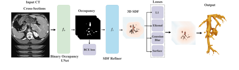 Figure 1. Overview of VesselSDF, our two-stage approach for vessel segmentation and reconstruction from CT scans. In the first stage, a 3D U-Net predicts a binary occupancy map. The second stage refines this occupancy into a signed distance field (SDF) using an additional 3D U-Net, guided by geometric regularization terms. The output 3D SDF, converted into a mesh, contains high-quality reconstructed vessels
-
Initial Input: Our particle $x$ starts its journey as a coordinate within a raw volumetric CT scan $V$. The system also has access to the local image features around $x$ from the CT scan.
-
Stage 1: Occupancy Prediction (The "Rough Sketch" Phase):
- The coordinate $x$ (or rather, the features extracted from the CT scan at and around $x$) first enters the 3D U-Net for Binary Occupancy Prediction, which we call $f_o(\cdot; \theta_o)$.
- Inside this U-Net, the input features are processed through an encoder-decoder structure. At various levels, 3D attention gates (as described in Equation 2) act like intelligent filters. They analyze the incoming feature maps, $g_e$ and $h_e$, and generate attention weights $a_e$. These weights then modulate the skip-connection features, ensuring that the network focuses its computational effort on salient vessel regions and preserves fine details that might otherwise be lost.
- After passing through this U-Net, our particle $x$ is assigned an occupancy probability, $f_o(x)$. This value, typically between 0 and 1, represents the network's initial "guess" as to whether $x$ belongs to a vessel (e.g., $f_o(x) \approx 1$) or the background (e.g., $f_o(x) \approx 0$). This is like getting a rough, binary sketch of the vessel.
-
Stage 2: SDF Refinement (The "Precision Sculpting" Phase):
- The occupancy probability $f_o(x)$ from Stage 1 is then passed to the SDF Refiner network, $f_r(\cdot; \theta_r)$. Crucially, the gradients from this stage are detached from the first stage's parameters (
detach(fo(x;θo))). This means the SDF refiner uses the occupancy prediction as a fixed input, preventing its own geometric constraints from interfering with the initial segmentation task. - The SDF Refiner, another 3D U-Net, takes this occupancy information and, through its own multi-resolution processing, transforms it into a continuous signed distance value, $f_{SDF}(x)$. This value is no longer a probability but a real number: negative if $x$ is inside a vessel, positive if outside, and ideally zero if exactly on the vessel surface. This is where the rough sketch is transformed into a precise, continuous geometric representation.
- The occupancy probability $f_o(x)$ from Stage 1 is then passed to the SDF Refiner network, $f_r(\cdot; \theta_r)$. Crucially, the gradients from this stage are detached from the first stage's parameters (
-
Loss Calculation (The "Quality Control" Phase):
- Now, both $f_o(x)$ and $f_{SDF}(x)$ are compared against their respective ground-truth values ($y$ for occupancy, $f^*_{SDF}(x)$ for SDF).
- The $\mathcal{L}_{occ}$ term checks how well $f_o(x)$ matches the true binary label $y$.
- The $\mathcal{L}_{sdf}$ term measures the absolute difference between $f_{SDF}(x)$ and the true SDF $f^*_{SDF}(x)$.
- The $\mathcal{L}_{eik}$ term scrutinizes the gradient of $f_{SDF}(x)$, ensuring it's close to 1, thus verifying that $f_{SDF}(x)$ behaves like a proper distance field.
- The $\mathcal{L}_{gauss}$ term applies a distance-weighted smoothing check to $f_{SDF}(x)$, making sure distant regions are smooth while preserving sharp details near the surface.
- Finally, the $\mathcal{L}_{sur}$ term penalizes any weak, ambiguous near-zero SDF values, effectively "cleaning up" potential floating artifacts.
- All these individual checks are combined into the total loss $\mathcal{L}$, which provides a single metric of the model's performance for our particle $x$.
-
Parameter Update (The "Learning" Phase):
- Based on the total loss $\mathcal{L}$, gradients are computed and used by the optimizer (Adam in this case) to adjust the parameters ($\theta_o$ and $\theta_r$) of both U-Nets. This iterative adjustment, repeated over many particles and epochs, allows the entire system to learn and improve its predictions.
-
Final Output (The "Reconstructed Vessel"):
- After training, for inference, the system takes new CT scan data, and for any point $x$, it outputs its predicted $f_{SDF}(x)$. The vessel surface is then simply defined as the collection of all points where $f_{SDF}(x) = 0$. This zero-level set can then be converted into a 3D mesh using algorithms like Marching Cubes, yielding the final, high-quality reconstructed vessel.
Optimization Dynamics
The VesselSDF model learns and converges by iteratively minimizing the total loss function $\mathcal{L}$ using the Adam optimizer. This process involves a sophisticated interplay of gradients and loss landscape shaping, guided by the various terms in the master equation.
-
Gradient Behavior:
- During each training iteration, the Adam optimizer calculates gradients of the total loss $\mathcal{L}$ with respect to all trainable parameters ($\theta_o$ for the occupancy U-Net and $\theta_r$ for the SDF refiner U-Net).
- The
detachoperation in Equation 3 is a critical aspect of the gradient flow. It ensures that the gradients from the SDF-specific loss terms ($\mathcal{L}_{sdf}$, $\mathcal{L}_{eik}$, $\mathcal{L}_{gauss}$, $\mathcal{L}_{sur}$) do not propagate back to update the parameters $\theta_o$ of the initial occupancy prediction network. This design choice isolates the initial segmentation task, allowing it to provide a stable, reliable starting point without being perturbed by the more complex geometric constraints of the SDF. Only the $\mathcal{L}_{occ}$ term contributes to updating $\theta_o$. - Conversely, all five loss terms contribute to updating $\theta_r$, the parameters of the SDF refiner. This means the SDF refiner is simultaneously learning to match the ground-truth SDF, enforce Eikonal properties, smooth distant regions, and suppress floating artifacts, all while building upon the initial occupancy prediction.
-
Loss Landscape Shaping: Each term in the master equation sculpts the multi-dimensional loss landscape in a specific way, guiding the optimization towards a desirable solution:
- $\mathcal{L}_{sdf}$ (L1 Loss): This term creates a "V-shaped" valley in the loss landscape centered around the ground-truth SDF values. The linear penalty ensures a consistent gradient magnitude (except at the exact minimum), which helps the optimizer efficiently move towards the true SDF values. Its robustness to outliers means that occasional noisy ground-truth labels won't drastically distort the landscape with extremely steep gradients.
- $\mathcal{L}_{occ}$ (Binary Cross-Entropy): For the occupancy network, this term shapes a landscape that strongly penalizes incorrect classifications. It creates steep slopes that push predicted probabilities towards 0 for background and 1 for vessel, making it "energetically favorable" for the model to make clear, confident binary decisions.
- $\mathcal{L}_{eik}$ (Eikonal Regularization): This is a powerful geometric constraint. It creates a landscape where predictions with gradient magnitudes close to 1 are favored, forming a "trough" along the ideal SDF manifold. Deviations from this unit gradient result in steep penalties, effectively "pushing" the model's predictions to conform to the properties of a true distance function. This prevents the SDF from collapsing or inflating unnaturally.
- $\mathcal{L}_{gauss}$ (Distance-weighted Gaussian Regularization): This term introduces an adaptive smoothing effect on the loss landscape. In regions far from the vessel surface (where $|f_{SDF}(x)|$ is large), this term creates a smoother, flatter landscape, encouraging the model to reduce high-frequency noise. However, near the vessel surface (where $|f_{SDF}(x)| \approx 0$), its influence is diminished, allowing the landscape to retain sharper features corresponding to fine vessel details. This is a clever way to balance global smoothness with local precision.
- $\mathcal{L}_{sur}$ (Surface Regularization): The exponential nature of this term creates a very steep "cliff" in the loss landscape around $f_{SDF}(x) = 0$. If the model predicts a weak, unsupported surface (i.e., $f_{SDF}(x)$ is close to zero but not strongly confirmed by other terms), this term generates a strong gradient that pushes $f_{SDF}(x)$ away from zero. This effectively "erases" spurious floating artifacts by making it highly unfavorable for the model to predict ambiguous near-surface values.
-
Iterative State Updates and Convergence:
- The Adam optimizer, with its adaptive learning rates for each parameter, efficiently navigates this complex loss landscape. It uses estimates of the first and second moments of the gradients to adjust the step size for each parameter, allowing for faster convergence in relevant directions and slower updates in noisy or flat regions.
- Over 100 epochs, the model iteratively updates its parameters. Initially, the predictions might be rough, but as training progresses, the combined influence of the supervised terms pulls the predictions towards the ground truth, while the regularization terms refine the geometry, ensuring smoothness, proper distance field properties, and the suppression of artifacts. The joint training, with the detached gradient flow, allows the model to first establish a robust occupancy map and then meticulously refine it into a high-quality, continuous SDF, leading to accurate and topologically coherent vascular reconstructions. The learning rate of $5 \times 10^{-4}$ is a common choice for Adam, providing a good balance between speed and stability.
Results, Limitations & Conclusion
Experimental Design & Baselines
The authors meticulously designed their experiments to validate the efficacy of VesselSDF, a two-stage framework for vascular network reconstruction. For the first stage, which predicts a binary occupancy map, they employed a 3D U-Net architecture enhanced with attention gates to capture multi-scale vessel features. The second stage, responsible for refining this occupancy into a continuous Signed Distance Field (SDF), utilized a lighter 3D U-Net with two encoder-decoder levels. Both stages were trained jointly for 100 epochs using the Adam optimizer with a learning rate of $5 \times 10^{-4}$. Notably, no data augmentation was applied during training to preserve the accuracy of SDF values. The training was conducted on whole-volume inputs of size $512 \times 512 \times 16$ with a batch size of 16. After reconstruction, marching cubes were applied at a resolution of 512 to extract the final vessel meshes. The total loss function, $\mathcal{L} = \lambda_s \mathcal{L}_{sdf} + \lambda_o \mathcal{L}_{occ} + \lambda_e \mathcal{L}_{eik} + \lambda_g \mathcal{L}_{gauss} + \lambda_{sur} \mathcal{L}_{sur}$, incorporated several terms: supervised SDF and occupancy losses, Eikonal regularization for smooth distance transitions, a distance-weighted Gaussian regularizer for adaptive smoothness, and surface regularization to suppress floating artifacts. The weights for these terms were set as $\lambda_s = 0.1$, $\lambda_o = 0.01$, $\lambda_e = 0.01$, $\lambda_g = 0.1$, and $\lambda_{sur} = 0.1$.
The "victims" (baseline models) against which VesselSDF was rigorously tested were three state-of-the-art volumetric segmentation architectures that perform binary voxel classification:
1. 3D-UNet [5]: A foundational encoder-decoder architecture widely used in medical image segmentation.
2. 3D SA-UNet [8]: An extension of 3D-UNet incorporating spatial attention modules, designed to adaptively weight feature responses, particularly beneficial for thin vasculature.
3. nnU-Net [9]: A self-configuring method that employs two U-Nets (one for low-resolution and one for higher-resolution processing) to achieve robust medical image segmentation.
VesselSDF's performance was evaluated on two public hepatic vessel segmentation datasets:
- Hepatic Vessels dataset (Medical Segmentation Decathlon - Task 08) [2]: Comprising 303 CT scans of hepatic veins with semi-automated annotations.
- IRCADb dataset [19]: Containing 20 contrast-enhanced abdominal CT scans with fully manual segmentations of liver vascular structures.
Ground truth SDFs were computed from the binary ground truth for training.
To definitively prove its mathematical claims, the authors used a comprehensive set of five metrics for 3D vessel reconstruction:
- Volumetric overlap: Dice Score and Volume IoU (Intersection over Union).
- Topological similarity: Jaccard Distance (JD).
- Geometric accuracy: Chamfer Distance (CD) and Hausdorff Distance (HD), which measure average and maximum surface distances, respectively.
What the Evidence Proves
The evidence presented in Table 1 and Fig. 2 unequivocally demonstrates the superior performance of VesselSDF, particularly in preserving the geometric fidelity and connectivity of complex vascular networks.
On the challenging Hepatic Vessels dataset, VesselSDF outperformed all baseline models across every single metric. For instance, its Dice score was 0.72 compared to nnU-Net's 0.69, and its Chamfer Distance (a lower value indicates better performance) was 0.68, significantly better then nnU-Net's 0.82. This is definitive, undeniable evidence that VesselSDF's core mechanism, leveraging continuous SDFs and geometric regularization, yields more accurate volumetric and surface reconstructions than traditional binary voxel classification.
For the IRCADb dataset, VesselSDF achieved comparable performance to the baselines on volume-based metrics (Dice, IoU, JD), indicating similar overall segmentation accuracy. However, it significantly outshone the baselines on surface-based metrics (CD and HD). For example, VesselSDF's CD was 0.60, while nnU-Net's was 0.75, and its HD was 3.5 compared to nnU-Net's 4.2. This highlights that while the overall volume might be similar, VesselSDF produces a much more geometrically precise and smooth vessel surface, which is crucial for clinical analysis.
Qualitative results in Fig. 2 further reinforce these findings. The visual comparisons clearly show that VesselSDF preserves thin vessels and complex branching paterns more effectively, leading to reconstructions that are more complete and anatomically coherent. The method demonstrably reduces common artifacts such as floating geometry and disconnected structures, which plague binary voxel classification approaches.
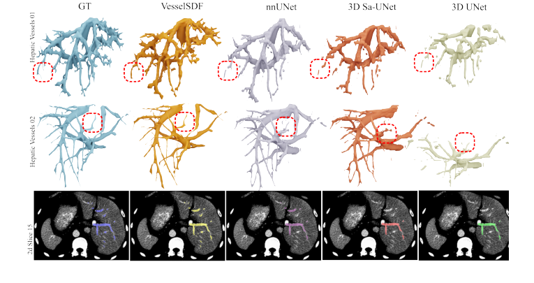 Figure 2. Qualitative 3D reconstruction results on the Hepatic Vessels dataset. The bottom row displays 2D slices highlighting the segmentation results
The ablation study in Table 2 provides crucial insights into the contribution of each component of VesselSDF. Removing the SDF refinement stage (w/o SDF refinement) led to a drop in Dice score from 0.72 to 0.69 and an increase in CD from 0.68 to 0.70, proving that the second stage is vital for geometric accuracy. Bypassing the initial binary occupancy prediction and directly predicting the SDF (w/o Binary Occupancy) resulted in an even more substantial performance degradation (Dice 0.65, CD 0.75), validating the benefit of the two-stage approach in separating vessel detection from geometric refinement. Finally, removing the adaptive Gaussian regularization (w/o Gaussian Loss) maintained similar Dice scores but introduced surface artifacts, confirming its role in ensuring global smoothness without over-smoothing critical vessel edges. The full VesselSDF achieves best performance across all metrics, with SDF refinement particularly enhancing vessel continuity as shown by the improved reconstruction metrix.
Limitations & Future Directions
While VesselSDF presents a significant advancement in vascular network reconstruction, particularly for sparse CT data, the paper implicitly points to areas for further development. The conclusion states that VesselSDF exhibits "fewer issues such as floating geometry and disconnected structures," implying that these challenges, while mitigated, might not be entirely eliminated. The focus on hepatic vessels and sparse CT slices also suggests potential limitations in generalization.
Here are some discussion topics for how we can further develop and evolve these findings:
-
Generalization Across Anatomies and Modalities: The current work focuses on hepatic vessels from CT scans. How robust is VesselSDF when applied to other complex vascular networks, such as coronary arteries, cerebral vasculature, or renal vessels, which may have different geometric characteristics and pathologies? Furthermore, how would it perform on different imaging modalities like MRA or CTA with varying resolutions and noise profiles? Could a more generalized "foundation model" for vascular reconstruction be developed, perhaps by incorporating diverse datasets and domain adaptation techniques?
-
Computational Efficiency and Real-time Applications: While SDFs offer high geometric fidelity, their computation and reconstruction can be resource-intensive. For clinical applications requiring rapid feedback, such as intraoperative guidance or real-time diagnostic support, the inference speed of VesselSDF might be a bottleneck. Future work could explore more efficient neural implicit representations, sparse SDF techniques, or optimized hardware acceleration to enable near real-time 3D reconstruction of vascular networks.
-
Integration with Advanced Clinical Workflows: Beyond static reconstruction, how can the high-quality 3D vessel models generated by VesselSDF be integrated into more advanced clinical workflows? This could involve simulating blood flow dynamics for hemodynamic analysis, precise surgical planning with augmented reality overlays, or even patient-specific device design. Developing user-friendly interfaces and tools that allow clinicians to interact with and analyze these continuous 3D representations would be crucial.
-
Robustness to Pathological Variations and Anomalies: The datasets used primarily represent typical vessel structures. Real-world clinical data often includes significant pathological variations such as severe stenoses, aneurysms, arteriovenous malformations, or tumor angiogenesis, which can drastically alter vessel morphology. How robust is VesselSDF to these extreme deviations from typical anatomy? Future research could focus on incorporating more diverse pathological datasets, developing loss functions that are sensitive to specific pathological features, or employing adversarial training to improve robustness against anomalous structures.
-
Uncertainty Quantification in Reconstruction: In medical imaging, knowing the confidence of a model's prediction is often as important as the prediction itself. For VesselSDF, especially in regions with high sparsity or noise, quantifying the uncertainty of the reconstructed SDF could provide valuable information to clinicians. Exploring Bayesian neural networks or ensemble methods to estimate uncertainty in the SDF prediction could enhance the clinical utility and trustworthiness of the reconstructions.
-
Beyond Static 3D: Towards 4D Reconstruction: Many vascular pathologies involve dynamic processes, such as vessel pulsatility, blood flow changes, or deformation over time. Could VesselSDF be extended to reconstruct 4D (3D + time) vascular networks from dynamic imaging sequences? This would open avenues for studying vessel mechanics, blood flow patterns, and the progression of diseases in a more comprehensive manner.
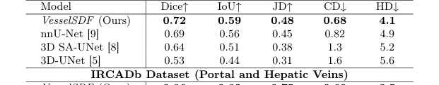 Table 1. Quantitative Results on the Hepatic Vessels and IRCADb datasets. Comparison of vessel reconstruction performance using different baselines. We report volume metrics (Dice Coefficient, Intersection over Union (IoU), and Jaccard similarity (JD)) and surface metrics (Chamfer distance (CD) ×100 and Hausdorff Distance (HD))
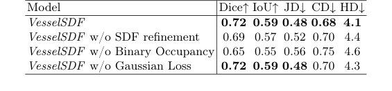 Table 2. Ablations on the Hepatic Vessels dataset