Dynamic behavior analysis of vegetation water model with double saturation transformation term

Background & Academic Lineage

The Origin & Academic Lineage

The problem of land desertification, a crucial environmental problem that is widely present in dry, semi-arid, and semi-humid regions, forms the precise origin of this research. It emrged in dry, semi-arid, and semi-humid regions globally due to natural factors and human activities accelerating desertification, leading to soil erosion, dwindling plant life, and compromised ecosystem stability. The academic field of mathematical ecology has sought to model these complex interactions.

Historically, Klausmeier [8] introduced a foundational vegetation-water system (model 1.1) that incorporated spatial diffusion and transport. This model served as a basis for subsequent research. For instance, Sherratt et al. [9] integrated an impulsive framework to study sporadic rainfall, and Consolo et al. [10] analyzed Turing patterns using a generalized hyperbolic Klausmeier model. Kealy et al. [11] simplified Klausmeier's model (leading to model 1.2) by removing convective terms and using linear diffusion, making it more applicable to flat terrains. This simplified model was further investigated by Sun et al. [12], Zhang et al. [13], and Gou et al. [14] to characterize stable configurations, bifurcation parameters, and parameter impacts on vegetation distribution. Li et al. [29] then introduced a water absorption saturation effect into the system (model 1.3), acknowledging that plants regulate water uptake physiologically, reaching a maximum absorption capacity at a certain biomass threshold.

The fundamental limitation, or "pain point," of these previous approaches, including model (1.3) with its single saturation term, was their inability to fully capture the bidirectional saturation interactions between vegetation and water. While model (1.3) accounted for vegetation's saturated water uptake, it did not explicitly model the saturation characteristics of water availability itself. This omission meant that earlier models provided a less vivid and biologically faithful depiction of the mutual influence and transformation relationship between vegetation and water, especially in desertification-prone regions where both water and vegetation can become limiting factors simultaneously. This gap forced the authors to develop the current papers' model, which incorporates a "double saturation transformation term" to address this crucial bidirectional feedback, thereby enhancing the model's biological fidelity despite increasing its analytical complexity.

Intuitive Domain Terms

• Land Desertification: Imagine a once-lush garden slowly turning into a barren, sandy patch. This happens when the soil loses its ability to support plant life, often due to a combination of natural dryness and human activities like overgrazing or deforestation. It's like the garden is slowly "drying up" and becoming a desert.
• Turing Instability: Think about a plain, uniformly colored cake batter. If you introduce certain ingredients (like specific chemicals in a reaction or diffusion rates in a biological system) and let them interact, the batter might spontaneously develop distinct, repeating patterns—like stripes, spots, or labyrinths—as it sets. Turing instability describes this phenomenon where a uniform state becomes unstable and give's rise to complex, organized patterns.
• Double Saturation Transformation Term: Consider a thirsty plant (vegetation) trying to drink from a water source. First, the plant itself can only absorb so much water, no matter how much is available (vegetation saturation). Second, if there's very little water in the soil to begin with, the plant can't absorb much, even if it's capable of absorbing more (water saturation). This "double saturation" term in the model accounts for both of these limits simultaneously, making the interaction more realistic.
• Bifurcation Phenomena: Picture a river flowing in a single, steady stream. If you gradually change a condition, like the slope of the land or the amount of water flowing, the river might suddenly split into two distinct channels, or start to meander dramatically, or even dry up. In mathematics, a bifurcation is when a small, continuous change in a system's parameter leads to a sudden, qualitative change in its behavior or the number and type of its solutions.

Notation Table

Notation	Description	Type
$w$	Non-dimensional water density	Variable
$n$	Non-dimensional vegetation biomass	Variable
$x$	Non-dimensional spatial coordinate	Variable
$t$	Non-dimensional time	Variable
$s$	Non-dimensional water yield (precipitation intensity)	Parameter
$p$	Non-dimensional parameter related to vegetation growth/water conversion	Parameter
$b$	Non-dimensional vegetation decrease rate	Parameter
$k$	Non-dimensional water saturation threshold	Parameter
$d_1$	Non-dimensional soil-water diffusion coefficient	Parameter
$d_2$	Non-dimensional vegetation diffusion coefficient	Parameter

Problem Definition & Constraints

Core Problem Formulation & The Dilemma

The core problem addressed by this paper is to develop a more biologically faithful mathematical model for vegetation-water interaction in desertification-prone regions. Previous models, such as Klausmeier's (1.1) and its extensions like Kealy et al.'s (1.2) and Li et al.'s (1.3), captured the saturation effect of vegetation's water absorption capacity, represented by a term like $F(N) = \frac{aN^2}{1+bN}$.

The Input/Current State is a set of existing vegetation-water models that, while foundational, do not fully capture the bidirectional saturation interactions between vegetation and water. Specifically, they lack a mechanism to account for the saturation of water availability itself, leading to a less realistic depiction of eco-hydrological feedback.

The Output/Goal State is a new vegetation-water system, specifically model (1.4) and its non-dimensional form (1.5), that incorporates double saturation transformation terms. This new model aims to more accurately and vividly describe the mutual influence and transformation relationship between vegetation and water, thereby enhancing its biological fidelity in representing moisture-vegetation interactions in desertification-prone areas. The ultimate goal is to enable a deeper and more realistic analysis of dynamic behaviors, including global stability, Turing instability, and various bifurcation phenomena, under these refined conditions.

The exact missing link or mathematical gap that this paper attempts to bridge lies in the saturation dynamics of water. While previous models considered the saturation of vegetation's water uptake ($F(N)$), they did not explicitly model the saturation of water itself. This paper introduces a water saturation function $G(W) = \frac{W}{W+K}$ (where $W$ is water density and $K$ is a saturation constant). The crucial innovation is the combined double saturation term $RG(W) \cdot F(N) \cdot N$ (or its non-dimensional equivalent $\frac{pwn^2}{(w+k)(n+1)}$). This term precisely characterizes the synergistic limitation of vegetation's saturated water absorption capacity and water's own saturation characteristics, providing a more accurate elucidation of nonlinear eco-hydrological feedback.

The painful trade-off or dilemma that has trapped previous researchers, and is explicitly highlighted by the authors, is the balance between biological realism and analytical tractability. The paper states: "The inclusion of the water saturation function G(W) substantially increases the model's biological fidelity, allowing it to more realistically describe the moisture-vegetation interaction in desertification-prone areas. However, it also raises the analytical complexity, particularly in deriving steady-state solutions and conducting bifurcation analysis, due to the introduction of higher-order nonlinearities." This means that achieving a more accurate biological representation comes at the significant cost of increased mathematical difficulty in solving and analyzing the system.

Constraints & Failure Modes

The problem of accurately modeling vegetation-water dynamics in desertification-prone regions is insanely difficult due to several harsh, realistic walls the authors hit:

• Physical and Ecological Constraints:

  • Non-negative Solutions: For any biological model, the densities of water ($w$) and vegetation ($n$) must remain non-negative. The system (1.5) is subject to non-negative initial data $(w_0(x,0), n_0(x,0)) \ge (0,0)$, which is a fundamental requirement for physical realism. Failure to maintain non-negativity would render the model biologically meaningless.
  • Bounded Domain and Zero-Flux Boundary Conditions: The analysis is conducted on a bounded spatial domain $\Omega$ with a smooth boundary, subject to zero-flux (Neumann) boundary conditions ($\frac{\partial w}{\partial \nu} = \frac{\partial n}{\partial \nu} = 0$ on $\partial \Omega$). These conditions represent a closed system where no water or vegetation crosses the boundaries, which is a realistic assumption for many ecological patches but adds complexity to the partial differential equations (PDEs).
  • Saturation Phenomena: The core of the problem involves accurately capturing the saturation of both vegetation's water uptake and water availability itself. This is a complex physiological and environmental reality that must be embedded in the model.
  • Environmental Factors: The model must implicitly or explicitly account for various natural factors (precipitation, wind velocity, light) and human activities (livestock farming) that influence vegetation distribution and water dynamics.

• Computational and Mathematical Constraints:

  • Higher-Order Nonlinearities: The introduction of the double saturation term $G(W) \cdot F(N)$ significantly increases the nonlinearity of the system (1.4) and its non-dimensional form (1.5). This makes the derivation of steady-state solutions, stability analysis, and bifurcation analysis substantially more challenging compared to linear or lower-order nonlinear systems. Standard analytical techniques often struggle with such high degrees of nonlinearity.
  • Analytical Complexity for Steady-State Solutions: Finding explicit steady-state solutions for highly nonlinear reaction-diffusion systems is generally very difficult. The paper relies on rigorous mathematical derivations, a priori estimates, and qualitative analyses, which are computationally intensive and require advanced mathematical tools.
  • Bifurcation Analysis Challenges: Analyzing bifurcation phenomena, especially those associated with simple and double eigenvalues, requires sophisticated methods like the Lyapunov-Schmidt reduction method and the Crandall-Rabinowitz theorem. These methods are intricate and their application becomes more involved with increased nonlinearity. The paper notes that for certain conditions (e.g., when $j \neq 2i$ and $i \neq 2j$), the implicit function theorem cannot be applied to establish the existence of solutions, indicating a failure mode for standard analytical approaches.
  • Turing Instability Conditions: Determining the conditions under which Turing instability occurs (leading to pattern formation) involves complex eigenvalue analysis of the linearized system, which is highly dependent on diffusion coefficients and other parameters.
  • Parameter Space Exploration: The model involves numerous parameters (e.g., $s, p, b, k, d_1, d_2$). Thoroughly investigating the influence of each parameter on the system's dynamic behavior and pattern formation requires extensive theoretical analysis and numerical simulations, making the problem space vast and difficult to fully explore. The paper's numerical simulations are essential to validate theoretical predictions across this complex parameter landscape.

Why This Approach

The Inevitability of the Choice

The authors of this paper faced a fundamental limitation with existing vegetation-water models: they failed to adequately capture the complex, bidirectional saturation effects between vegetation and water in desertification-prone regions. Traditional models, such as the Klausmeier model (system 1.1) and its extensions (like system 1.3 by Li et al.), primarily incorporated a single saturation term, typically describing how vegetation's water absorption capacity saturates as its biomass increases, represented by a function like $f(N) = \frac{aN^2}{1+bN}$.

However, the authors realized that this was insufficient. The exact moment of this realization is articulated on page 3, where they state: "To better capture the bidirectional saturation interactions between vegetation and water in desertification-prone regions, we further refine system (1.3) by incorporating a double saturation transforma- tion mechanism." This highlights that the problem isn't just about vegetation absorbing water, but also about the water's own saturation characteristics and how that simultaneously limits vegetation growth. Without accounting for both, the models were missing a crucial piece of the ecological puzzle. Therefore, a model incorporating double saturation terms was not merely an improvement but the only viable solution to accurately represent these intricate, mutual limitations. This was a clear shortcomming.

Comparative Superiority

The qualitative superiority of this approach stems directly from its enhanced biological fidelity, rather than just improved performance metrics in a computational sense. The introduction of the "double saturation transformation terms" via the new nonlinear coupling term $RG(W) \cdot F(N) \cdot N$ is the key structural advantage. This term, as explained on page 3, "characterizes the simultaneous limitation of water and vegetation in absorption dynamics."

Previous models, by only considering single saturation, could not fully represent this synergistic limitation. The inclusion of the water saturation function $G(W)$ alongside the vegetation absorption rate $F(N)$ allows the model to "more realistically describe the moisture-vegetation interaction in desertification-prone areas" and "more accurately elucidating the nonlinear mechanism of eco-hydrological feedbak." This means the model isn't just fitting data better; it's structurally designed to mirror the real-world ecological processes more faithfully. It provides a deeper, more nuanced understanding of how these two critical components interact under stress, which is a significant qualitative leap over prior gold standards. The paper does not discuss aspects like handling high-dimensional noise or reducing memory complexity, as its focus is on the foundational mathematical modeling of ecological phenomena.

Alignment with Constraints

To be honest, I’m not completely sure about the specific constraints defined in Step 2, as that section was not provided. However, based on the problem definition and motivation presented in the paper, we can infer several harsh requirements that this chosen method perfectly addresses. The core problem revolves around accurately modeling vegetation-water interactions in "desertification-prone regions" (Abstract, Page 3), which implies a need for high fidelity in capturing critical feedback mechanisms under environmental stress.

The "marriage" between the problem's requirements and the solution's unique properties is evident in several ways:
1. Realistic Depiction of Mutual Influence: The problem demands a model that "more vividly depicts the mutual influence and transformation relationship between vegetation and water" (Abstract). The double saturation terms, $G(W)$ and $F(N)$, directly fulfill this by explicitly modeling how both water availability and vegetation's absorption capacity simultaneously limit each other.
2. Bidirectional Saturation Interactions: The authors explicitly sought to "better capture the bidirectional saturation interactions between vegetation and water" (Page 3). The novel double saturation term $RG(W) \cdot F(N) \cdot N$ is precisely designed for this, ensuring that the model accounts for saturation from both sides of the interaction, which was a critical missing piece in previous models.
3. Elucidating Nonlinear Mechanisms: Desertification involves complex, nonlinear eco-hydrological feedback. The chosen method, with its higher-order nonlinearities introduced by the double saturation terms, allows for "more accurately elucidating the nonlinear mechanism of eco-hydrological feedback in desertification-prone areas" (Page 3). This aligns perfectly with the need to understand the intricate dynamics that drive pattern formation and ecosystem stability in these vulnerable environments.

Rejection of Alternatives

The paper's reasoning for rejecting alternative approaches is primarily implicit and focused on the limitations of previous mathematical models rather than entirely different methodological paradigms like GANs or Transformers. The authors build upon a lineage of reaction-diffusion models, starting with Klausmeier's system (1.1) and its subsequent extensions (e.g., Kealy et al.'s system (1.2), Li et al.'s system (1.3)).

The core reason for rejecting these earlier models as sufficient is their inability to capture the "bidirectional saturation interactions between vegetation and water" (Page 3). While these models incorporated a single saturation term (e.g., $f(N) = \frac{aN^2}{1+bN}$ for vegetation water uptake), they lacked a corresponding term for water saturation, $G(W)$. The authors found that "traditional" methods, in this context meaning single-saturation vegetation-water models, were "insufficient for this specific problem" because they could not "simultaneously capture the saturation effects of both vegetation's water absorption capacity and water availability itself" (Page 4). This omission led to a less realistic depiction of eco-hydrological feedbak. Therefore, the new model, with its double saturation terms, was introduced as a necessary refinement to overcome these specific shortcomings of its predecessors within the same modeling framework. The paper does not delve into why machine learning models like GANs or Diffusion models would fail, as they operate on a different level of abstraction and are not directly comparable to the mechanistic differential equation modeling approach taken here.

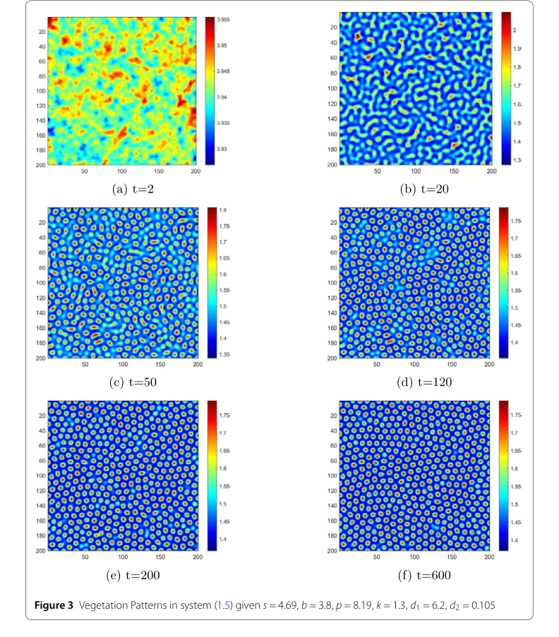Figure 3. Vegetation Patterns in system (1.5) given s = 4.69, b = 3.8, p = 8.19, k = 1.3, d1 = 6.2, d2 = 0.105

Mathematical & Logical Mechanism

The Master Equation

The absolute core of this paper's mathematical engine is the non-dimensionalized reaction-diffusion system, which describes the dynamic interaction between vegetation biomass and water density. This system, derived from the original model by incorporating double saturation transformation terms and then scaled, is presented as:

$$ \begin{cases} \frac{\partial w}{\partial t} = s - w - \frac{pwn^2}{(w+k)(n+1)} + d_1\Delta w, & x \in \Omega, t > 0, \\ \frac{\partial n}{\partial t} = \frac{pwn^2}{(w+k)(n+1)} - bn + d_2\Delta n, & x \in \Omega, t > 0, \\ \frac{\partial w}{\partial \nu} = \frac{\partial n}{\partial \nu} = 0, & x \in \partial\Omega, t > 0, \\ (w_0(x, 0), n_0(x, 0)) \geq, \neq (0,0), & x \in \Omega. \end{cases} $$

Term-by-Term Autopsy

Let's dissect this master equation piece by piece to understand its components and their roles:

• $w$:

  • Mathematical Definition: A dependent variable representing the non-dimensionalized density of water. It's a scalar field, meaning its value can vary across space and time.
  • Physical/Logical Role: This term quantifies the amount of water available in the ecosystem at any given location $x$ and time $t$.
  • Why used: It's the primary state variable for water.

• $n$:

  • Mathematical Definition: A dependent variable representing the non-dimensionalized density of vegetation biomass. Like $w$, it's a scalar field.
  • Physical/Logical Role: This term quantifies the amount of vegetation biomass present at any given location $x$ and time $t$.
  • Why used: It's the primary state variable for vegetation.

• $t$:

  • Mathematical Definition: The independent variable representing time.
  • Physical/Logical Role: This is the temporal dimension over which the system evolves.
  • Why used: To describe how $w$ and $n$ change over time.

• $x \in \Omega, t > 0$:

  • Mathematical Definition: Specifies the domain for the partial differential equations (PDEs). $\Omega$ is a bounded spatial region, and $t > 0$ means we are looking at the system's evolution after the initial moment.
  • Physical/Logical Role: Defines the physical space and time interval where the model applies.
  • Why used: To set the context for the spatial and temporal dynamics.

• $\frac{\partial w}{\partial t}$:

  • Mathematical Definition: The partial derivative of water density $w$ with respect to time $t$.
  • Physical/Logical Role: This represents the instantaneous rate of change of water density at a specific point in space. A positive value means water is increasing, negative means it's decreasing.
  • Why used: To model the temporal evolution of water.

• $\frac{\partial n}{\partial t}$:

  • Mathematical Definition: The partial derivative of vegetation biomass density $n$ with respect to time $t$.
  • Physical/Logical Role: This represents the instantaneous rate of change of vegetation biomass at a specific point in space.
  • Why used: To model the temporal evolution of vegetation.

• $s$:

  • Mathematical Definition: A positive constant parameter.
  • Physical/Logical Role: Represents the constant input of water into the system, analogous to precipitation or rainfall. It's a source term for water.
  • Why used: To model a continuous external supply of water. It's an additive term because it directly contributes to the water pool.

• $-w$:

  • Mathematical Definition: A linear term, the negative of the water density.
  • Physical/Logical Role: Represents the rate of water loss due to evaporation. In the original dimensional model, this was $LW$, where $L$ is the evaporation rate. After non-dimensionalization, $L$ is implicitly absorbed or set to 1. It's a sink term for water.
  • Why used: To model water loss proportional to its presence. It's a subtractive term because water is removed from the system.

• $-\frac{pwn^2}{(w+k)(n+1)}$ (in the first equation):

  • Mathematical Definition: A complex nonlinear term involving $p, w, n, k$.
  • Physical/Logical Role: This is the crucial "double saturation transformation term" that represents the rate at which vegetation absorbs water. The $p$ is a conversion efficiency. The $n^2$ suggests that water absorption increases more than linearly with vegetation density, possibly due to cooperative effects or increased surface area. The denominators $(w+k)$ and $(n+1)$ introduce saturation: as water $w$ or vegetation $n$ become very high, the rate of water absorption doesn't increase indefinitely but approaches a maximum. This term is subtracted from the water equation because water is consumed by vegetation.
  • Why used: To capture the realistic biological phenomenon of water uptake by vegetation, including saturation effects for both water availability and vegetation's absorption capacity. Multiplication combines the influences of $p, w, n^2$. Division by $(w+k)$ and $(n+1)$ creates the saturation effect, where the rate flattens out at high values, which is a common way to model limited resources or capacities in biology.

• $+d_1\Delta w$:

  • Mathematical Definition: A diffusion term, where $d_1$ is a positive constant and $\Delta$ is the Laplace operator ($\Delta w = \frac{\partial^2 w}{\partial x_1^2} + \frac{\partial^2 w}{\partial x_2^2} + \dots$).
  • Physical/Logical Role: Represents the spatial spreading of water due to diffusion (e.g., infiltration through soil, lateral flow). Water tends to move from areas of higher concentration to lower concentration, smoothing out spatial differences. The positive sign indicates this smoothing effect.
  • Why used: To model the natural tendency of water to disperse in space. It's an additive term because it represents a net flux that can increase or decrease local water density depending on the curvature of the water profile.

• $\frac{pwn^2}{(w+k)(n+1)}$ (in the second equation):

  • Mathematical Definition: Identical nonlinear term as in the first equation.
  • Physical/Logical Role: This term represents the rate at which vegetation grows by converting the absorbed water into biomass. It's a source term for vegetation.
  • Why used: To link water absorption directly to vegetation growth. It's an additive term because this process increases vegetation biomass.

• $-bn$:

  • Mathematical Definition: A linear term, product of $b$ and $n$. $b$ is a positive constant.
  • Physical/Logical Role: Represents the natural death or loss rate of vegetation biomass. It's a sink term for vegetation.
  • Why used: To model the natural decay or mortality of vegetation. It's a subtractive term because vegetation is removed from the system.

• $+d_2\Delta n$:

  • Mathematical Definition: A diffusion term, where $d_2$ is a positive constant and $\Delta$ is the Laplace operator applied to $n$.
  • Physical/Logical Role: Represents the spatial spreading of vegetation (e.g., through asexual reproduction, seed dispersal). Vegetation tends to spread from areas of higher density to lower density.
  • Why used: To model the natural dispersal of vegetation in space. It's an additive term for the same reasons as $d_1\Delta w$.

• $\frac{\partial w}{\partial \nu} = \frac{\partial n}{\partial \nu} = 0, x \in \partial\Omega, t > 0$:

  • Mathematical Definition: Neumann boundary conditions, where $\frac{\partial}{\partial \nu}$ denotes the normal derivative (the rate of change perpendicular to the boundary).
  • Physical/Logical Role: These conditions impose a "zero-flux" or "no-flow" constraint at the boundaries of the spatial domain. This means no water or vegetation biomass enters or leaves the system across its edges.
  • Why used: To define a closed system where all interactions occur within the specified domain, preventing external influences from affecting the boundary dynamics.

• $(w_0(x, 0), n_0(x, 0)) \geq, \neq (0,0), x \in \Omega$:

  • Mathematical Definition: Initial conditions for water and vegetation densities. They are non-negative and not identically zero everywhere.
  • Physical/Logical Role: Specifies the starting spatial distribution of water and vegetation biomass at the initial time $t=0$. The non-zero condition ensures there is an initial "seed" for the dynamics to unfold.
  • Why used: To provide a starting point for the simulation or analysis of the system's evolution.

Step-by-Step Flow

Imagine a tiny, abstract parcel of water and a small patch of vegetation coexisting at a specific location within our ecological domain. Let's trace their journey through the mathematical engine:

1. Water Inflow: First, the water parcel receives a constant, steady supply of water, $s$, akin to precipitation. This is its primary input.
2. Water Loss (Evaporation): Simultaneously, a portion of the water in the parcel is lost to the environment through evaporation, represented by the $-w$ term. The more water there is, the more evaporates.
3. Vegetation's Thirst (Water's Perspective): Next, the vegetation patch at this location begins to absorb water from the parcel. This absorption is a complex process: it's driven by the vegetation's density ($n^2$) and an efficiency factor ($p$), but it's also limited. As the water parcel becomes very wet (high $w$) or the vegetation patch becomes very dense (high $n$), the rate of absorption doesn't keep increasing indefinitely; it "saturates" or levels off, thanks to the $(w+k)$ and $(n+1)$ terms in the denominator. This absorbed water is removed from the water parcel.
4. Water Spreading: After these local interactions, the water in the parcel doesn't stay put. It diffuses, spreading out to neighboring areas, while water from adjacent areas also diffuses into this parcel. This process, governed by the diffusion coefficient $d_1$ and the Laplace operator $\Delta w$, acts like a smoothing mechanism, tending to equalize water concentrations across space.
5. Vegetation Growth (Vegetation's Perspective): Now, let's switch to the vegetation patch. The very same water that was absorbed from the parcel (the $\frac{pwn^2}{(w+k)(n+1)}$ term) is converted into new vegetation biomass. This is the vegetation's primary growth mechanism, directly linking its expansion to water availability and its own density. This new biomass is added to the vegetation patch.
6. Vegetation Loss (Mortality): However, vegetation also faces natural losses. A portion of the vegetation biomass, proportional to its current density ($bn$), dies off or is lost due to other factors. This is subtracted from the vegetation patch.
7. Vegetation Spreading: Similar to water, vegetation biomass also spreads spatially. Driven by the diffusion coefficient $d_2$ and the Laplace operator $\Delta n$, vegetation disperses into less dense areas, and new vegetation spreads into this patch from neighbors.
8. Boundary Containment: At the very edges of the entire ecological domain, a "zero-flux" condition is imposed. This means no water or vegetation can flow in or out across these boundaries, effectively making the system a self-contained unit.
9. Continuous Evolution: These steps don't happen sequentially but continuously and simultaneously at every single point in the domain. Over time, starting from an initial distribution of water and vegetation, this intricate interplay of local reactions (inflow, evaporation, absorption, growth, loss) and spatial diffusion causes the entire ecosystem to evolve, potentially leading to stable uniform states or complex, dynamic spatial patterns.

Optimization Dynamics

In the context of this reaction-diffusion system, "optimization dynamics" refers not to a model learning from data or minimizing a loss function in a machine learning sense, but rather to how the system evolves and converges to stable states or patterns over time. The "learning" here is the system's intrinsic tendency to find its natural configurations.

1. Evolution Towards Equilibria: The system's primary dynamic is to evolve towards equilibrium points where the rates of change for both water and vegetation become zero ($\frac{\partial w}{\partial t} = 0$ and $\frac{\partial n}{\partial t} = 0$). These equilibria represent steady states where the inputs and outputs, and the reaction and diffusion processes, are perfectly balanced. The paper identifies several such points: a "boundary equilibrium" (e.g., a state with only water and no vegetation) and "positive equilibria" (states with both water and vegetation).

2. Stability and the "Loss Landscape": The concept of a "loss landscape" can be intuitively mapped to the stability landscape of these equilibria. If an equilibrium is stable, the system, when slightly perturbed, will tend to return to that state. If it's unstable, even a tiny perturbation will cause the system to move away. The shape of this landscape is determined by the nonlinear interactions and diffusion terms. The paper uses linear stability analysis by examining the eigenvalues of the Jacobian matrix of the linearized system around an equilibrium.

   • For a homogeneous equilibrium, if all eigenvalues have negative real parts, it's stable. If any eigenvalue has a positive real part, it's unstable.

3. Turing Instability: Pattern Formation: A key dynamic is Turing instability, which is how spatial patterns emerge. This occurs when a spatially uniform equilibrium is stable to uniform perturbations (meaning it would return to homogeneity if disturbed evenly) but becomes unstable to spatially varying perturbations (meaning certain spatial wavelengths of disturbance grow).

   • The diffusion coefficients ($d_1$ and $d_2$) are critical here. If they are sufficiently different, they can destabilize the uniform state for specific spatial frequencies, leading to the spontaneous formation of patterns like spots, stripes, or gaps. This is like the system "finding" a more complex, spatially heterogeneous "optimum" in its state space. The paper analyzes this by looking at how the eigenvalues of the linearized system (which now include diffusion terms) behave for different spatial wavenumbers.

4. Bifurcation Dynamics: Qualitative Shifts: As key parameters (like the water diffusion coefficient $d_1$) are varied, the system can undergo bifurcations. This means the qualitative nature of the solutions changes dramatically. For instance, a stable uniform state might suddenly give rise to stable spatial patterns, or vice versa.

   • The paper investigates steady-state bifurcations, where new equilibrium solutions (often non-uniform patterns) branch off from existing ones. The direction of these bifurcations (supercritical or subcritical) determines if the new patterns are stable and emerge smoothly (supercritical) or are unstable and appear abruptly (subcritical), potentially leading to hysteresis. This is determined by higher-order derivatives of the bifurcation function.

5. Iterative State Updates (Numerical Simulation): While the mathematical analysis provides theoretical insights into stability and bifurcation, the actual "iterative updates" of the system's state over time are visualized through numerical simulations. The partial differential equations are solved computationally by discretizing space and time. At each small time step, the values of $w$ and $n$ at every spatial grid point are updated based on the local reaction terms and the diffusion from neighboring points. This iterative process allows researchers to observe the emergence and evolution of spatial patterns, confirming the theoretical predictions and illustrating how the system "converges" to its dynamic configurations. The figures in the paper vividly demonstrate this, showing how initial random noise evolves into organized spots, stripes, or gap patterns under different parameter settings.

Results, Limitations & Conclusion

Experimental Design & Baselines

The experimental validation of the theoretical findings in this study was conducted through numerical simulations of the proposed vegetation-water system (1.5). The primary objective was to ruthlessly prove the mathematical claims regarding stability, instability, and pattern formation. The authors architected their experiments by selecting two distinct parameter configurations, each designed to align with specific theoretical predictions.

For the first set of parameters, chosen to demonstrate local asymptotic stability, the values were set as $s = 4.69$, $p = 8.19$, $k = 1.3$, $b = 3.8$, $d_1 = 6$, and $d_2 = 0.105$. These parameters were specifically selected to satisfy the condition $z < \dot{z} < z_2$, which, according to Theorem 2.2, predicts the local asymptotic stability of the equilibrium point $(w_1, n_1)$.

Conversely, for the second set of parameters, intended to illustrate Turing instability, the values were $s = 4.69$, $p = 8.19$, $k = 1.3$, $b = 3.8$, $d_1 = 6$, and $d_2 = 0.05$. This configuration was chosen to meet the conditions $d_2\lambda_1 < \frac{b}{n_1+1}$ and $d_1 > \bar{d_1}$, which, as per Theorem 2.5 (2), should lead to the Turing unstable state of the equilibrium point $(w_1, n_1)$.

The simulations were performed on a two-dimensional spatial region defined as $[0,50] \times [0,50]$ and evolved over a time interval of $[0,600]$ seconds. The initial conditions for these simulations involved introducing small random perturbations to the stationary solutions $(w_1, n_1)$ within a spatially homogeneous system. The "victims" in this experimental design were not external baseline models, but rather the theoretical predictions themselves. The definitive evidence of the core mechanism's work was the direct visual and quantitative confirmation that the numerical simulations accurately reproduced the predicted stable or unstable behaviors and the subsequent pattern formations.

What the Evidence Proves

The numerical simulations provided undeniable evidence that the core mathematical mechanism, particularly the role of double saturation terms and diffusion coefficients, worked as predicted by the theoretical analyses.

1. Validation of Stability and Instability:
   • Local Asymptotic Stability: For the first parameter set, Figure 1 graphically illustrates the evolution of the system. The "u1 Value" (water density) and "u2 Value" (vegetation biomass) plots show that, despite initial perturbations, the system quickly converges to a uniform, stable state across the spatial domain over time. This directly validates Theorem 2.2, confirming that under specific conditions, the equilibrium point $(w_1, n_1)$ is indeed locally asymptotically stable.

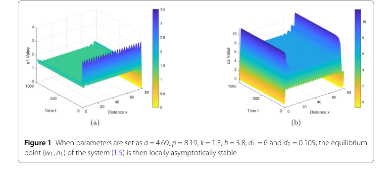Figure 1. When parameters are set as a = 4.69, p = 8.19, k = 1.3, b = 3.8, d1 = 6 and d2 = 0.105, the equilibrium point (w1,n1) of the system (1.5) is then locally asymptotically stable

*   **Turing Instability:** With the second parameter set, Figure 2 starkly contrasts the stable behavior. Here, the "u1 Value" and "u2 Value" plots clearly show the emergence and persistence of complex spatial patterns rather than a uniform state. This definitive pattern formation is the hallmark of Turing instability, providing hard evidence for the predictions of Theorem 2.5 (2). The system, initially perturbed, evolves into a structured, non-homogeneous state, proving that the theoretical conditions for instability were accurately identified.
*

Figure 2. When parameters are set as a = 4.69, p = 8.19, k = 1.3, b = 3.8, d1 = 6 and d2 = 0.05, the equilibrium point (w1,n1) of system (1.5) is Turing unstable

1. Dynamic Vegetation Pattern Formation:

   • Figure 3, illustrating vegetation distribution over time, reveals a fascinating sequence of pattern evolution. Starting from random perturbations, the system initially exhibits erratic, non-uniform temporary patterns. As time progresses (e.g., from $t=2$ s to $t=50$ s), stripe-like patterns begin to emerge. Eventually, by $t=600$ s, these evolve into dominant gap patterns, which then remain unchanged. This dynamic progression from initial disorder to stable, complex patterns provides compelling evidence of the model's ability to capture realistic ecological phenomena. The visual distinction between blue (low moisture) and red (high moisture) areas further elucidates the spatial distribution of resources.

2. Influence of Key Ecological Parameters:

   • Water Diffusion Coefficient ($d_1$): In Fig. 4 the first key factor is the water diffusion coefficient d₁. When d₁ = 3, as illustrated in Fig. 4 (a), regular, high-density spots emerge. Under these conditions water diffusion is slow, and vegetation grows in small, concentrated patches, like grassland patches in nature. As d₁ increases, transitioning to the scenario in Fig. 4 (b), the pattern evolves into complex labyrinthine stripes, high-water/low-vegetation and low-water/high-vegetation regions alternate. When d₁ reaches 5, the stripes elongate, forming a complex mix of bands and spots; enhanced water diffusion stretches the vegetation, making it more dispersed. When d₁ is set to 6.2, as shown in Fig. 4 (d), large, sparse patches appear. High-water regions expand widely, pushing vegetation into isolated small areas, causing vegetation density to decline. This sequence rigorously proves that increased moisture mobility (higher d₁) promotes vegetation dispersal and reduces biomass density.

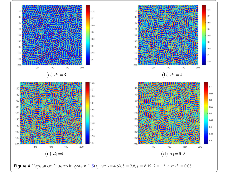Figure 4. Vegetation Patterns in system (1.5) given s = 4.69, b = 3.8, p = 8.19, k = 1.3, and d2 = 0.05

*   **Precipitation Intensity ($s$):** Figure 5 illustrates the effect of rainfall rate. Initially, with rising $s$ (e.g., $s=3.69$ to $s=4$), stripe patterns appear. Further increases in $s$ (e.g., $s=4.5$ to $s=4.69$) lead to the formation of gap patterns. This evidence proves a non-linear relationship between precipitation and vegetation growth, where higher rainfall rates, within a specific range, result in higher vegetation density but also drive transitions between different pattern types.
*   **Environmental Stress/Resource Competition ($p$):** Figure 6 shows that as parameter $p$ (associated with environmental stress or resource competition) slowly rises, the vegetation patterns, while maintaining their stripe-like structure, become narrower and more concentrated. This demonstrates that increased stress or competition leads to a more compact and less expansive vegetation distribution.

In summary, the numerical simulations not only validated the theoretical predictions of stability and instability but also provided a rich visual tapestry of dynamic pattern formations. This hard evidence, derived from systematically varying key parameters, definitively proved that the model's core mechanism, incorporating dual saturation terms, accurately captures the complex eco-hydrological feedback observed in desertification-prone enviroment.

Limitations & Future Directions

While this study presents a rigourous and insightful analysis of a novel vegetation-water model, it's important to acknowledge its inherent limitations and consider avenues for future development.

One immediate limitation stems from the increased nonlinearity introduced by the dual saturation terms. As the authors note, this significantly raises the analytical complexity, particularly in deriving steady-state solutions and conducting bifurcation analysis. While the paper successfully navigates these challenges, the computational intensity and mathematical intricacy could be a barrier for broader application or for incorporating even more complex ecological interactions. Future research could explore advanced numerical techniques or machine learning approaches to efficiently handle such high-order nonlinearities, potentially enabling faster simulations and broader parameter space exploration.

The scope of the numerical simulations is another point for discussion. The experiments were conducted on a specific two-dimensional spatial domain ($[0,50] \times [0,50]$) and a finite time interval ($[0,600]$). While sufficient for validating the theoretical claims, the generalizability of these findings to much larger geographical scales, longer ecological timescales, or different boundary conditions remains an open question. Future work could involve scaling up these simulations to regional or continental levels, perhaps by integrating with Geographic Information Systems (GIS) data, to assess the model's predictive power in real-world, heterogeneous landscapes.

Furthermore, the model, while advanced, primarily focuses on vegetation-water interactions. Other critical ecological factors influencing desertification, such as varying soil types, topography, grazing pressure from livestock, fire regimes, or the impact of different plant species (e.g., grasses vs. shrubs), are not explicitly detailed in the model's core equations. Incorporating these elements could lead to an even more comprehensive and realistic representation of desertification dynamics. For instance, how would the observed patterns change if soil water retention varied spatially, or if grazing pressure was introduced as a dynamic variable? This could lead to a multi-species vegetation model or a model with spatially explicit environmental heterogeneity.

The initial conditions for the simulations involved "small random perturbations." It would be valuable to investigate the system's behavior under larger or more structured perturbations, which might better mimic real-world disturbances like extreme weather events or human interventions. This could reveal different transient dynamics or alternative stable states not captured by small perturbations.

Looking forward, several discussion topics emerge from these findings:

• Predictive Modeling and Early Warning Systems: Given the model's ability to generate diverse spatial patterns mirroring observed vegetation dynamics, how can this be leveraged to develop predictive tools for desertification? Can specific pattern transitions (e.g., from spots to stripes to gaps) serve as early warning indicators for ecosystem degradation in semi-arid regions? This would require extensive calibration with long-term ecological monitoring data.
• Optimizing Resource Management: The insights into how water diffusion ($d_1$) and precipitation ($s$) influence vegetation patterns are crucial. How can these findings inform sustainable water allocation strategies in water-scarce regions? For example, understanding the critical $d_1$ values that lead to sparse patches could guide land managers in implementing measures to enhance soil water retention or reduce runoff, thereby promoting more resilient vegetation structures.
• Impact of Climate Change Scenarios: Beyond simple changes in precipitation intensity, how would the model respond to more complex climate change projections, such as increased frequency and intensity of droughts, shifts in seasonal rainfall patterns, or rising temperatures affecting evaporation rates? Integrating climate model outputs into this framework could provide valuable insights into future desertification risks.
• Cross-Disciplinary Collaboration: To truly evolve these findings, closer collaboration with field ecologists, hydrologists, and remote sensing experts is essential. Validating the model's predictions against empirical data from various desertification-prone regions would strengthen its ecological relevance and practical applicability. This could also involve using remote sensing data to infer vegetation patterns and water availability, which could then be used to calibrate and refine model parameters.
• Stochasticity and Uncertainty: The paper mentions previous work incorporating stochasticity [23]. How would the double saturation model behave under stochastic environmental fluctuations, reflecting the inherent uncertainty and variability in natural systems? This could provide a more robust understanding of vegetation resilience under unpredictable conditions.
• Bifurcation Analysis in Higher Dimensions: While the paper delves into local and global bifurcation analysis, the complexity of the model means that a full analytical treatment of all bifurcation phenomena in higher-dimensional spatial settings remains a significant challenge. Further theoretical advancements in this area could unlock deeper understanding of the model's rich dynamics.

By addressing these limitations and exploring these future directions, the foundational work presented in this paper can be significantly expanded, contributing to more effective strategies for combating desertification and promoting ecological resilience.