Compute-Constrained Data Selection
The field of large language models (LLMs) has seen explosive growth, leading to models with billions of parameters capable of remarkable feats in natural language understanding and generation.
Background & Academic Lineage
The field of large language models (LLMs) has seen explosive growth, leading to models with billions of parameters capable of remarkable feats in natural language understanding and generation. However, this power comes at a significant computational cost. Training these massive models, or even adapting them for specific tasks through a process called finetuning, requires immense computational resources, often measured in terms of Graphics Processing Unit (GPU) hours or FLOPs (Floating Point Operations).
The precise origin of the problem addressed in this paper stems from the practical reality of these resource constraints. As LLMs became more prevalent, researchers and practitioners quickly realized that the total compute budget for training or finetuning is often predetermined and fixed in advance. This means that the number of accelerators (like GPUs) and their usage hours are allocated upfront. This realization spurred research into "compute-optimal LLMs," where the goal is to achieve the best possible model performance (e.g., lowest perplexity) within a given computational budget. Early work, such as Hoffmann et al. (2022), explored how to balance architectural choices and training decisions to achieve this.
This paper extends this line of inquiry specifically to the finetuning phase of LLMs. A promising strategy to reduce the compute requirements for finetuning is "data selection," where instead of training on the entire available dataset, a smaller, more impactful subset is chosen. Data selection itself is a foundational concept in machine learning, with roots going back to the late 1960s (Hart, 1968) and 1970s (John, 1975), aiming to create minimal datasets for effective training.
However, the fundamental limitation or "pain point" of previous approaches that forced the authors to write this paper is that they largely ignored the computational cost of the data selection process itself. While data selection methods were designed to reduce the training data size (and thus training compute), many of the "powerful" or "sophisticated" selection methods require significant computational effort to identify the best data points. The core problem is that "even if data selection is effective, it does not a priori imply that it is compute-optimal." Previous models focused on maximizing performance for a given data budget (i.e., number of data points), but not necessarily for a given compute budget that encompasses both selection and training costs. This oversight meant that a method that selects the "best" data might be so expensive to run that the overall compute budget is better spent simply training on more data with a cheaper, or even random, selection strategy. The authors argue that for practical adoption, a compute-optimal method must both improve training and be cheap to compute, a critical factor that has been underconsidered.
Here are 3 to 5 highly specialized domain terms from the paper, translated into intuitive, everyday analogies for a zero-base reader:
- LLMs (Large Language Models): Imagine a super-smart digital assistant that has read almost everything ever written by humans. It can understand your questions, write stories, summarize articles, and even help you code, all by predicting the next most likely word.
- Finetuning: Think of it like this: you have a brilliant, general-purpose chef (the LLM) who knows how to cook all kinds of cuisines. Now, you want them to become an expert in baking French pastries. You give them a specific cookbook on French pastries and have them practice only those recipes. They don't forget how to cook other things, but they become much better at French pastries.
- Compute-Optimal: This is like trying to get the "best bang for your buck" when you're building something. You have a fixed amount of money (compute budget) and you want to achieve the highest quality result (model performance). It's about making smart choices on where to spend your money to get the most value, not just spending on the most expensive or seemingly "best" parts.
- Perplexity: Imagine you're trying to guess the next word in a sentence. If the sentence is "The cat sat on the...", you're not very surprised if the next word is "mat" or "rug." Your "perplexity" is low. But if the next word was "banana," you'd be very surprised, and your "perplexity" would be high. In LLMs, lower perplexity means the model is better at predicting text and understands the language more fluently.
- FLOPs (Floating Point Operations): These are the basic arithmetic calculations (like addition, subtraction, multiplication, division) that a computer performs. When we talk about FLOPs, it's like counting every single time a calculator button is pressed. It's a way to measure how much "thinking" or "work" a computer does. A higher FLOP count means more computational effort.
Notation Table
| Notation | Description |
|---|---|
| LLMs | Large Language Models, pre-trained on vast text data. |
| Finetuning | The process of adapting a pre-trained LLM to a specific downstream task using a smaller, task-specific dataset. |
| Compute Budget ($\mathcal{K}$) | The total, fixed computational resources (e.g., FLOPs, GPU hours) allocated for both data selection and model training. |
| FLOPs | Floating Point Operations, a measure of computational work. |
| $\mathcal{D}$ | The entire available pool of potential training data. |
| $\mathcal{S}$ | A subset of data selected from $\mathcal{D}$ for finetuning. |
| $\mathcal{S}^*$ | The optimal subset of data selected from $\mathcal{D}$ that maximizes model performance under compute constraints. |
| $P(\cdot)$ | A function representing the performance of an LLM on a given task (e.g., accuracy, perplexity). |
| $\mathcal{T}(\mathcal{S})$ | The LLM model trained (finetuned) on the data subset $\mathcal{S}$. |
| $\mathcal{T}$ | The target test dataset used for final evaluation of model performance. |
| $\mathcal{V}$ | The validation dataset, used as a proxy for $\mathcal{T}$ during data selection and model development. |
| $C_T(\mathcal{S})$ | The computational cost (in FLOPs) of training the LLM on the selected data subset $\mathcal{S}$. |
| $C_U(x)$ | The computational cost (in FLOPs) of computing the utility function for a single data point $x$ during the data selection process. |
| $\sum_{x \in \mathcal{D}} C_U(x)$ | The total computational cost of computing utility functions for all data points in the original dataset $\mathcal{D}$ to perform data selection. |
| $K$ (in traditional problem) | The maximum cardinality (number of data points) allowed in the selected subset $\mathcal{S}$ (a data budget). |
| $K$ (in compute-constrained problem) | The total compute budget (in FLOPs) for both data selection and training. |
| $v(x; \mathcal{V})$ | A utility function that assigns a score to data point $x$ based on its relevance or value, often computed with respect to the validation set $\mathcal{V}$. |
| $P_0$ | The zero-shot performance of the LLM (performance without any finetuning). |
| $P$ | The upper bound on performance, representing the maximum achievable performance. |
| $\lambda$ | A parameter in the parametric performance model that controls how efficiently a data selection method extracts value from additional compute. |
| $C(k)$ | The total computational cost (selection + training) for a strategy that results in training on $k$ data points. |
| $C(|\mathcal{D}|)$ | The total computational cost of training on the entire dataset $\mathcal{D}$ (without any data selection). |
| $\exp(\cdot)$ | The exponential function, used to model diminishing returns. |
| Levenberg-Marquardt | An algorithm used for solving non-linear least squares problems, employed here to fit the parameters of the parametric performance model. |
| LoRA | Low-Rank Adaptation, a parameter-efficient finetuning method that reduces memory usage. |
| QLoRA | Quantized LoRA, a further optimization for memory reduction, especially for very large models. |
| MMLU | Massive Multitask Language Understanding, a benchmark for factual knowledge. |
| BBH | Big-Bench Hard, a benchmark for complex reasoning. |
| IFEval | Instruction Following Evaluation, a benchmark for instruction following abilities. |
| BM25 | A Lexicon-Based data selection method, using statistical properties of text. |
| Embed | An Embedding-Based data selection method, using dense embedding models. |
| PPL | A Perplexity-Based data selection method, using LLM loss (perplexity). |
| LESS | A Gradient-Based data selection method, using gradients to estimate influence. |
Problem Definition & Constraints
The core problem this paper tackles revolves around optimizing the finetuning of Large Language Models (LLMs) under a strict, predetermined total compute budget.
The starting point (Input/Current State) is a scenario where we have:
* A vast pool of potential training data, denoted as $\mathcal{D}$.
* A specific downstream task for which a base LLM needs to be finetuned.
* Associated test ($\mathcal{T}$) and validation ($\mathcal{V}$) datasets to evaluate performance.
* A fixed, overall computational budget, $\mathcal{K}$, typically measured in FLOPs (Floating Point Operations), which represents the total resources allocated for both data selection and subsequent model training. This budget is often set in advance, for instance, by the number of accelerators and their usage hours.
* A variety of existing data selection methods, each with its own computational cost and effectiveness in identifying valuable training data.
The desired endpoint (Output/Goal State) is to identify an optimal subset of data, $\mathcal{S}^* \subset \mathcal{D}$, such that when an LLM is finetuned on this subset, $\mathcal{T}(\mathcal{S}^*)$, it achieves the highest possible performance $P(\mathcal{T}; \mathcal{T}(\mathcal{S}^*))$ on the target test set. Crucially, this optimal performance must be attained while adhering to the total compute budget $\mathcal{K}$, meaning the combined computational cost of selecting $\mathcal{S}^*$ and training on it must not exceed $\mathcal{K}$. The ultimate goal is to provide practitioners with a framework to make informed decisions on how to best allocate their finite compute resources between data selection and model training.
The exact missing link or mathematical gap this paper attempts to bridge lies in moving from a data-centric optimization to a compute-centric one. Traditionally, data selection problems are formulated as:
$$ \mathcal{S}^* = \arg \max_{\mathcal{S} \subset \mathcal{D}} P(\mathcal{T}; \mathcal{T}(\mathcal{S})) \quad \text{subject to } |\mathcal{S}| \le K $$
Here, $K$ represents a data budget (maximum number of data points). This formulation implicitly assumes that the cost of selecting the data is negligible or handled separately.
This paper introduces a new, more realistic formulation that explicitly incorporates the computational cost of data selection into the overall budget constraint. The problem is reframed as:
$$ \mathcal{S}^* = \arg \max_{\mathcal{S} \subset \mathcal{D}} P(\mathcal{V}; \mathcal{T}(\mathcal{S})) \quad \text{subject to } C_T(\mathcal{S}) + \sum_{x \in \mathcal{D}} C_U(x) \le \mathcal{K} $$
where:
* $P(\mathcal{V}; \mathcal{T}(\mathcal{S}))$ is used as a proxy for $P(\mathcal{T}; \mathcal{T}(\mathcal{S}))$, leveraging the validation set $\mathcal{V}$.
* $C_T(\mathcal{S})$ is the computational cost of training the model on the selected subset $\mathcal{S}$.
* $\sum_{x \in \mathcal{D}} C_U(x)$ is the total computational cost of computing the utility function $v(x; \mathcal{V})$ for all data points in the original dataset $\mathcal{D}$ to identify the subset $\mathcal{S}$.
* $\mathcal{K}$ is the total compute budget.
The mathematical gap is precisely the inclusion of the $\sum_{x \in \mathcal{D}} C_U(x)$ term in the constraint, transforming the optimization from being solely about data quantity to being about total compute expenditure.
The painful trade-off or dilemma that has trapped previous researchers is the inherent conflict between the effectiveness of a data selection method and its computational cost. More sophisticated data selection methods, such as those based on model perplexity or gradients, are often highly effective at identifying a smaller, high-quality subset of data that can lead to better model performance or faster convergence during training. However, these "powerful" methods are also significantly more compute-intensive to execute.
The dilemma is that while these advanced methods reduce the training data size, the substantial compute required for the selection process itself can easily outweigh the gains from reduced training time. In a fixed total compute budget scenario, spending more FLOPs on selection means fewer FLOPs are available for the actual finetuning process, potentially leading to worse overall performance despite having a "better" data subset. Researchers previously focused on maximizing performance for a given data size, not necessarily for a given total compute budget, thus overlooking this critical trade-off.
The harsh, realistic walls that make this problem insanely difficult to solve are multifaceted:
- Computational Intractability of Optimal Selection: The problem of finding the absolute optimal data subset $\mathcal{S}^*$ is a combinatorial optimization problem. Exhaustively searching all possible subsets is computationally infeasible for large datasets, making exact solutions impractical. This forces reliance on greedy algorithms and approximations.
- High Cost of LLM Operations: Finetuning LLMs, even with parameter-efficient methods like LoRA, is inherently compute-intensive. Each gradient step, forward pass, or backward pass through a large transformer model consumes a vast number of FLOPs. This makes both the $C_T(\mathcal{S})$ and $C_U(x)$ terms substantial.
- Varying Costs of Selection Methods: Different data selection methods have drastically different computational footprints. Lexicon-based methods (like BM25) are very cheap (near 0 FLOPs), embedding-based methods are moderately expensive (e.g., $4.4 \times 10^{16}$ FLOPs for Embed), while perplexity-based and gradient-based methods are extremely costly (e.g., $1.53 \times 10^{18}$ FLOPs for PPL, $8.27 \times 10^{18}$ FLOPs for LESS, as shown in Table 5). This wide range means that a method that is "best" in terms of data reduction might be "worst" in terms of total compute efficiency.
- Scaling Laws and Diminishing Returns: The efficacy of data selection often scales with the compute invested in it, but with diminishing returns. More compute might yield a slightly better subset, but the performance gains might not justify the additional cost. The relationship between compute and performance is non-linear and complex, as modeled by the parametric function $P(k) = (P - P_0) \times (1 - \exp(-\frac{\lambda C(k)}{C(|\mathcal{D}|)})) + P_0$.
- Proxy Reliance: The true objective $P(\mathcal{T}; \mathcal{T}(\mathcal{S}))$ cannot be directly optimized because the test set $\mathcal{T}$ is unavailable during selection. Researchers must rely on a validation set $\mathcal{V}$ and utility functions $v(x; \mathcal{V})$ as proxies, which introduces potential inaccuracies and assumptions (e.g., $\mathcal{V}$ being IID with $\mathcal{T}$).
- Model and Task Dependency: The optimal compute allocation and the "best" data selection method are not universal. They depend on the specific LLM size (e.g., 7B, 13B, 70B parameters), the nature of the downstream task (e.g., MMLU, BBH, IFEval), and the total compute budget available. This makes finding a general solution quite hard.
- Hardware Memory Limits: While not the central focus, the paper mentions using QLoRA for 70B models to reduce memory requirements (Appendix D.1), indicating that memory constraints are a practical wall in scaling LLM finetuning, which indirectly influences compute allocation strategies.
In essence, the problem is insanely difficult because it requires navigating a complex, non-linear optimization landscape where the "best" choice is highly context-dependent, and the very act of improving one aspect (data quality) can inadvertently cripple another (total compute efficiency).
Why This Approach
The core problem this paper addresses is the practical challenge of finetuning Large Language Models (LLMs) under a predetermined, finite computational budget. Traditionally, data selection methods have focused on optimizing model performance for a given data budget—meaning, selecting the best subset of a fixed size $K$ from a larger dataset $D$. The objective, as described in Section 3, is to find a subset $S^*$ that maximizes performance $P(T; T(S))$ on a test set $T$, subject to $|S| \le K$.
The authors realized that this traditional approach was insufficient for real-world LLM finetuning. The "exact moment" of this realization is clearly articulated in Section 4: "While the framework presented in Section 3 provides a general method for data selection, we argue that it is insufficient for the practical challenge of finetuning LLMs. The issue is that LLM finetuning is often bottlenecked by a computational budget and not a data budget." They observed that the total compute budget is often fixed in advance (e.g., allocated accelerators and usage hours), and this budget must cover both the cost of selecting the data and the cost of training the model on that selected data. Previous "SOTA" methods for data selection, while effective at identifying high-quality data subsets, often incurred substantial computational costs themselves, which were largely ignored in their evaluation.
The paper's approach isn't to introduce a new data selection algorithm, but rather a new, compute-constrained framework for evaluating and selecting data selection methods. This framework is the only viable solution for making truly optimal decisions in a compute-limited environment because it explicitly accounts for the total computational expenditure. The authors formalize this problem as:
$$S^* = \arg \max_{S \subset D} P(V; T(S)) \quad \text{subject to} \quad C_T(S) + \sum_{x \in D} C_U(x) \le K$$
Here, $K$ represents the total compute budget (e.g., maximum FLOPs), $C_T(S)$ is the cost of training the model on the selected subset $S$, and $\sum_{x \in D} C_U(x)$ is the cost of computing the utility function for data selection across the entire dataset $D$. This is a fundamental shift from optimizing for a fixed data size to optimizing for a fixed total compute.
Comparative Superiority (The Benchmarking Logic):
The qualitative superiority of this compute-constrained framework lies in its holistic and practical evaluation metric. The previous "gold standard" implicitly assumed infinite or negligible compute for data selection, focusing solely on the performance achieved by the selected data. This new framework, however, provides a Pareto frontier (as seen in Figures 2, 3, 5, 7, 8) that maps total compute (x-axis) to model performance (y-axis). This allows for a direct comparison of methods based on their efficiency in converting compute into performance, rather than just their raw performance on a fixed-size dataset.
This framework doesn't inherently handle high-dimensional noise better or reduce memory complexity of the underlying data selection algorithms. Instead, its structural advantage is that it reveals the true compute-optimal methods under various budget scenarios. It demonstrates that methods with lower computational complexity for selection (like Lexicon-Based BM25 or Embedding-Based) often become overwhelmingly superior to more sophisticated, compute-intensive methods (like Perplexity-Based PPL or Gradient-Based LESS) when the total compute budget is limited. For instance, the abstract notes that "cheaper data selection alternatives dominate both from a theoretical and empirical perspective." This is a profound qualitative advantage: it changes which methods are considered "best" by introducing a critical real-world constraint. The conceptual behavior of these methods under varying compute budgets is illustrated in a simulation.
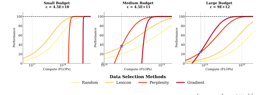 Figure 1. Simulation of Performance under Constraints. P(k) = ¯P × ? 1 −exp ? −λ C(k)
Alignment with Constraints ("Marriage"):
The "marriage" between the problem's harsh requirements and the solution's unique properties is perfect. The problem's harsh requirements, as stated in the introduction, are:
1. Predetermined total compute budget: LLM training is expensive, and resources (accelerators, usage hours) are allocated upfront.
2. Optimal resource allocation: It's critical to determine how to best allocate this fixed budget.
3. Data selection must be compute-optimal: Any data selection method must improve training in proportion to its added cost.
The compute-constrained objective (Equation 2) directly addresses these requirements:
* It sets a strict upper bound $K$ on the total compute, forcing a trade-off between selection cost and training cost.
* It quantifies the "added cost" of data selection ($C_U(x)$) and integrates it with the training cost ($C_T(S)$), enabling practitioners to make informed decisions about resource allocation.
* It allows for the identification of methods that are truly "compute-optimal" by considering the entire pipeline, not just isolated parts. This ensures that the chosen method is not only effective but also economically viable within the given computational limits. This framework is a direct response to the practical need for efficiency in a resource-constrained world.
Rejection of Alternatives:
The paper implicitly "rejects" traditional "SOTA" data selection methods, such as Perplexity-Based (PPL) and Gradient-Based (LESS), when compute is constrained. It does not discuss alternatives like GANs or Diffusion models, as its scope is specifically data selection for finetuning.
The reasoning for rejecting these otherwise powerful methods is their high computational cost for selection, which makes them FLOP-inefficient under a total compute budget.
* High Cost: Section 4.1 and Appendix B provide clear evidence. Lexicon-Based (BM25) costs approximately $1 \times 10^8$ FLOPs, and Embedding-Based (Embed) costs around $4.4 \times 10^{16}$ FLOPs. In stark contrast, Perplexity-Based (PPL) costs about $1.53 \times 10^{18}$ FLOPs, and Gradient-Based (LESS) costs a staggering $8.27 \times 10^{18}$ FLOPs. These are orders of magnitude more expensive.
* FLOP Inefficiency: The abstract and Section 7 explicitly state that "many powerful data selection methods are almost never compute-optimal" and that PPL and LESS are "FLOP inefficient both from a theoretical and empirical perspective."
* Empirical Failure: Figures 1 and 2 demonstrate this. For small and medium compute budgets, the cheaper BM25 and Embed methods consistently outperform PPL and LESS on the compute-performance Pareto frontier. This means that for a given total compute budget, one can achieve better model performance by using a cheaper selection method and allocating more compute to actual model training.
* Break-Even Point: The paper finds that PPL and LESS only become compute-optimal when the training model is significantly larger than the selection model (5x for PPL, 10x for LESS, as detailed in Section 8 and Appendix G). This implies that for most practical scenarios where the selection model is of comparable size or smaller relative to the training model, these sophisticated methods would have failed to be compute-optimal. The marginal benefit of their superior data selection quality simply does not outweigh their exorbitant computational cost.
Mathematical & Logical Mechanism
As a Meta-scientist, I've thoroughly reviewed the provided paper, "COMPUTE-CONSTRAINED DATA SELECTION," which tackles a crucial challenge in the era of large language models (LLMs): how to optimally allocate a fixed computational budget between selecting training data and actually finetuning the model. The authors present a compelling analysis, demonstrating that simply choosing the most "powerful" data selection method isn't always the most compute-efficient approach.
Before diving into the paper's specifics, let's establish some foundational concepts:
- Large Language Models (LLMs): Imagine an incredibly smart digital assistant that can understand and generate human-like text. These are LLMs. They are "large" because they have billions of internal parameters (like knobs) and are trained on vast amounts of text data (like the entire internet). This training process is immensely expensive and time-consuming.
- Finetuning: Once an LLM is pre-trained, it's a generalist. To make it good at a specific task (e.g., answering medical questions, writing code), we "finetune" it. This involves training it further on a smaller, task-specific dataset. It's like teaching a general-purpose chef to specialize in French cuisine.
- Compute Budget: Think of this as your total allowance for computational resources. It's measured in FLOPs (Floating Point Operations), which are basic arithmetic calculations. Training LLMs requires a lot of FLOPs, often involving expensive hardware like GPUs running for days or weeks. This budget is often fixed beforehand.
- Data Selection: Instead of finetuning on all available task-specific data (which can still be huge), data selection is the process of intelligently picking a smaller, more impactful subset of that data. The idea is that not all data points are equally valuable, and some might even be redundant or harmful. Selecting the "best" data can make finetuning faster and more effective.
- Performance: How well the LLM does on its target task after finetuning. This could be measured by accuracy, how coherent its generated text is, or other metrics.
- Diminishing Returns: This is a common economic principle: the more you invest in something, the smaller the additional benefit you get from each subsequent investment. For example, the first few hours of studying for an exam might yield huge improvements, but the 100th hour might only give a tiny boost. This applies to compute and data in LLM training.
The central motivation of this paper stems from a practical dilemma:
- LLM finetuning is expensive: Training these massive models, even for specific tasks, consumes significant computational resources.
- Data selection can help: By picking a smaller, high-quality dataset, we can reduce the amount of training compute needed. This sounds great!
- But data selection itself costs compute: To figure out which data points are "best," you often need to run some calculations, sometimes even using another LLM. This process isn't free.
The authors realized that previous work often focused on data selection's effectiveness in reducing data size or improving performance per training step, but it didn't fully account for the computational cost of the selection process itself. A data selection method might be "powerful" (meaning it picks great data), but if it costs a huge amount of compute to run, it might not be the most efficient choice when you have a strict total compute budget.
The problem the authors set out to solve is this: Given a fixed total compute budget, how should a practitioner optimally balance the compute spent on selecting data versus the compute spent on training the model on that selected data, to achieve the highest possible model performance? They want to quantify this trade-off and identify truly "compute-optimal" strategies.
Constraints That Had to Be Overcome
The authors faced several practical and theoretical constraints:
- Fixed Total Compute Budget ($K$): This is the overarching constraint. All computational efforts, from evaluating data points for selection to the actual model training, must fit within this predetermined limit. It's like having a fixed amount of money for a project, and you need to decide how much to spend on planning (data selection) versus execution (training).
- Computational Cost of Data Selection ($C_U(x)$): Different data selection methods have vastly different computational footprints. Some are cheap (e.g., simple text statistics), while others are very expensive (e.g., running forward/backward passes on an LLM). This cost is often incurred for every data point in the original, large dataset to determine its utility, even if only a small subset is ultimately chosen. This "overhead" can quickly eat into the total budget.
- Computational Cost of Training ($C_T(S)$): Even with a selected subset $S$, training still requires compute. This cost scales with the size of the selected data and the size of the LLM being finetuned.
- Limited Access to the True Test Set ($T$): In real-world scenarios, the ultimate test set (the data the model will be evaluated on after deployment) is typically not available during the data selection phase. Therefore, the authors had to rely on a validation set ($V$) as a proxy for evaluating performance during the selection process. This introduces a potential gap between proxy performance and true performance.
- Combinatorial Complexity: Choosing the absolute best subset of data from a large pool is a combinatorial optimization problem, meaning the number of possible subsets is astronomically large. Directly searching for the optimal subset is computationally infeasible. The authors address this by using greedy approximations (scoring all points and picking the best) and then modeling the performance with a parametric function.
- Modeling Diminishing Returns: The relationship between compute and performance is not linear. Initial compute investments yield high returns, but these returns diminish as more compute is added. Accurately modeling this non-linear behavior was crucial for their analysis.
The paper presents two key mathematical formulations. The first defines the problem itself, and the second is a parametric model used to analyze and understand the compute-performance relationship.
The Master Equation: Problem Formulation
The absolute core problem that this paper addresses is formalized as finding the optimal subset of data points $S^*$ from a larger dataset $D$ that maximizes the performance of a finetuned model, subject to a total computational budget $K$.
$$S^* = \arg \max_{S \subset D} P(V; \mathcal{T}(S))$$
$$\text{subject to } C_T(S) + \sum_{x \in D} C_U(x) \le K$$
Tear the equation apart:
- $S^*$:
1) Mathematical Definition: This denotes the optimal subset of data points.
2) Physical/Logical Role: This is the ultimate goal of the entire process: the specific collection of training examples that, when used, will yield the best model performance given the compute constraints. It's the "answer" to the data selection problem.
3) Why $\arg \max$: We are not just interested in the maximum performance value itself, but in which subset $S$ achieves that maximum performance. "Arg max" means "the argument (in this case, $S$) that maximizes the expression." - $P(V; \mathcal{T}(S))$:
1) Mathematical Definition: This is the performance metric of the model $\mathcal{T}(S)$, which has been trained (finetuned) on the data subset $S$, evaluated on the validation set $V$.
2) Physical/Logical Role: This term represents the quality or effectiveness of the finetuned model. It's the objective we want to maximize. A higher value here means a better model. The validation set $V$ acts as a stand-in for the true, unseen test data, allowing us to estimate performance during the selection process. - $S \subset D$:
1) Mathematical Definition: This indicates that $S$ must be a subset of the original, large training dataset $D$.
2) Physical/Logical Role: This defines the search space. We are choosing data points from the available pool $D$, not creating new ones. The core idea of data selection is to reduce the amount of data, so $S$ is typically much smaller than $D$. - $C_T(S)$:
1) Mathematical Definition: This is the computational cost (measured in FLOPs) required to train the model $\mathcal{T}$ on the selected data subset $S$.
2) Physical/Logical Role: This is the "training cost" component of our total compute budget. It's the compute spent on actually teaching the model using the chosen data. This cost typically increases with the size of $S$ and the complexity of the model.
3) Why addition: This cost is added to the data selection cost because both activities consume resources from the same overall compute budget. They are two parts of a single expenditure. - $\sum_{x \in D} C_U(x)$:
1) Mathematical Definition: This is the sum of the computational costs $C_U(x)$ for computing the utility (or "score") of every single data point $x$ in the entire original dataset $D$.
2) Physical/Logical Role: This represents the "data selection cost" overhead. For many data selection methods, you first need to evaluate all potential data points to decide which ones are most valuable. This sum is the fixed computational investment required to perform the selection, regardless of how many points are ultimately chosen for training. It's the cost of "shopping" for the best data.
3) Why summation: The utility cost is calculated for each individual data point, and these individual costs are then summed up to get the total cost for the utility computation phase. The authors use a summation over $D$ because, in their greedy approach, they score all points in $D$ to select the best $K$. - $K$:
1) Mathematical Definition: This is the total maximum computational budget (in FLOPs) that is available for both data selection and model training.
2) Physical/Logical Role: This is the hard resource constraint. It's the "bank account balance" that cannot be exceeded. The entire problem revolves around maximizing performance within this budget.
3) Why $\le$: The total compute used must be less than or equal to the allocated budget. We cannot spend more compute than we have.
The Master Equation: Performance Model for Analysis
To analyze the trade-off and understand how performance changes with compute, the paper introduces a parametric model for expected performance $P(k)$ after training on $k$ data points. This model is used to fit empirical data and extrapolate findings.
$$P(k) = (P - P_0) \times \left(1 - \exp\left(-\frac{\lambda C(k)}{C(|\mathcal{D}|)}\right)\right) + P_0$$
Tear the equation apart (for the performance model):
- $P(k)$:
1) Mathematical Definition: The expected performance of the model after training on $k$ selected data points.
2) Physical/Logical Role: This is the predicted performance value. It's the output of our model, telling us how well the LLM is expected to perform given a certain amount of compute and selected data. This is what's plotted on the y-axis of the performance graphs. - $P$:
1) Mathematical Definition: The upper bound on performance.
2) Physical/Logical Role: This represents the maximum possible performance the model can achieve on the task, even if trained on the entire dataset $D$. It's the "ceiling" or "ideal" performance that the model asymptotically approaches. - $P_0$:
1) Mathematical Definition: The zero-shot performance.
2) Physical/Logical Role: This is the baseline performance of the model before any finetuning. It's the starting point from which all performance gains are measured. - $(P - P_0)$:
1) Mathematical Definition: The total potential performance gain.
2) Physical/Logical Role: This term scales the exponential growth. It represents the maximum possible improvement we can get from finetuning, from the baseline $P_0$ up to the ceiling $P$. - $\times$:
1) Mathematical Definition: Multiplication.
2) Physical/Logical Role: This operator scales the fractional gain (from the exponential term) by the total potential performance improvement.
3) Why multiplication: The exponential term calculates a fraction of the total potential gain that has been achieved. Multiplying it by $(P - P_0)$ converts this fraction into an absolute performance gain. - $1 - \exp\left(-\frac{\lambda C(k)}{C(|\mathcal{D}|)}\right)$:
1) Mathematical Definition: An exponential growth function that starts at 0 and approaches 1.
2) Physical/Logical Role: This is the core "learning curve" component. It models the diminishing returns. For small compute, this term grows rapidly, indicating significant performance gains. As compute increases, its growth slows down, reflecting that each additional unit of compute yields less and less additional performance. The exponential function is a natural choice for modeling such saturation behavior.
3) Why exponential: Exponential functions are excellent for modeling processes that exhibit diminishing returns or saturation, where the rate of change decreases as the input increases. - $\exp(\cdot)$:
1) Mathematical Definition: The exponential function $e^x$.
2) Physical/Logical Role: Used to create the diminishing returns curve. - $-$ (inside $1 - \exp$):
1) Mathematical Definition: Subtraction.
2) Physical/Logical Role: The term $\exp(-x)$ starts at 1 and decays towards 0. By subtracting this from 1, we get a function $1 - \exp(-x)$ that starts at 0 and grows towards 1, which is suitable for representing an achieved fraction of the total potential gain. - $\lambda$:
1) Mathematical Definition: A positive scalar parameter.
2) Physical/Logical Role: This is the "efficiency" parameter. It dictates how effectively a particular data selection method (and its associated training) converts compute into performance gain. A larger $\lambda$ means the method is more efficient, achieving higher performance for the same amount of compute, making the learning curve steeper.
3) Why multiplication: $\lambda$ directly scales the effective compute, making the method more or less sensitive to the compute investment. - $C(k)$:
1) Mathematical Definition: The total computational cost of selecting $k$ data points and training on them. This is calculated as $c \times k + \sum_{x \in D} C_U(x)$, where $c$ is the cost per data point for training.
2) Physical/Logical Role: This is the actual compute spent for a given strategy. It combines the cost of data selection and training. It's the "input" to the performance function, representing the total investment.
3) Why division: It's part of a ratio, normalizing the actual compute spent against the total compute for full training. - $C(|\mathcal{D}|)$:
1) Mathematical Definition: The total computational cost of training on the entire dataset $D$ (without any data selection).
2) Physical/Logical Role: This serves as a normalization factor for the compute cost $C(k)$. It puts $C(k)$ into context relative to the cost of "doing nothing" (i.e., training on all available data without selection).
3) Why division: Normalizes $C(k)$ to a dimensionless ratio, making the exponential term more general and interpretable as a fraction of total possible compute. - $+$ (outside $\exp$):
1) Mathematical Definition: Addition.
2) Physical/Logical Role: This operator shifts the entire performance curve upwards by the zero-shot performance $P_0$. This ensures that when no effective compute is used (or $k=0$), the predicted performance starts at the baseline $P_0$.
3) Why addition: The exponential term calculates the gain above $P_0$. To get the absolute performance, this gain is added to the baseline $P_0$.
Step-by-step Flow: Tracing an Abstract Data Point (through the Performance Model)
Let's imagine we're evaluating a specific data selection strategy and want to predict its performance. This isn't about a single data point flowing through the LLM, but rather how the total compute associated with a strategy translates into a performance prediction using the parametric model.
- Strategy Definition: We start by choosing a specific data selection method (e.g., "Perplexity-Based") and decide on a target number of data points ($k$) we want to select for finetuning.
- Calculate Data Selection Overhead: The chosen data selection method first needs to compute a "utility score" for every single data point in the original, large dataset $D$. This involves a fixed computational cost, $\sum_{x \in D} C_U(x)$, which is like the initial "setup fee" for using this method.
- Determine Training Cost: Based on the chosen $k$ data points (which would be the top $k$ points after scoring all of $D$), we calculate the cost of training the LLM on this specific subset. This is $c \times k$, where $c$ is the cost per data point.
- Aggregate Total Compute ($C(k)$): We sum these two costs: $C(k) = (c \times k) + \sum_{x \in D} C_U(x)$. This $C(k)$ is the total computational investment for this particular strategy (using this method to select $k$ points and then training on them).
- Normalize Compute Investment: This total compute $C(k)$ is then divided by a reference cost: $C(|\mathcal{D}|)$, which is the cost of simply training on the entire original dataset $D$ without any selection. This gives us a normalized ratio, indicating how much compute we're spending relative to a "full" training run.
- Apply Method Efficiency ($\lambda$): The normalized compute ratio is then multiplied by $\lambda$, a parameter unique to the chosen data selection method. This $\lambda$ acts as a "booster" or "attenuator," reflecting how efficiently this specific method translates compute into performance gains. A method with a high $\lambda$ gets more "bang for its buck" from the compute.
- Compute Performance Gain Factor: The result from step 6 is fed into the exponential term: $1 - \exp\left(-\frac{\lambda C(k)}{C(|\mathcal{D}|)}\right)$. This function starts at 0 and curves upwards, gradually approaching 1. It mathematically captures the idea of diminishing returns: initially, small increases in compute lead to large jumps in this factor, but as compute grows, the factor increases more slowly.
- Scale by Potential Improvement: This gain factor is then multiplied by the total potential performance improvement, $(P - P_0)$. This converts the abstract gain factor into a concrete amount of performance points gained above the baseline.
- Add Baseline Performance: Finally, the zero-shot performance $P_0$ (the model's performance before any finetuning) is added to the calculated gain. This gives us the final predicted absolute performance $P(k)$ for the chosen strategy.
This entire process is repeated for various data selection methods and different numbers of selected data points ($k$), generating a series of performance curves. By comparing these curves, the authors can identify which method is "compute-optimal" for different total compute budgets.
Optimization Dynamics: How the Mechanism Learns, Updates, or Converges
The paper doesn't describe an iterative learning process for the LLM itself (like gradient descent to update model weights). Instead, it focuses on two levels of "optimization":
-
Learning the Performance Landscape (Parameter Fitting): The primary "learning" mechanism described in the paper is the process of fitting the parameters ($P_0, P, \lambda$) of the parametric performance model (Equation 3) to the observed empirical data.
- Loss Landscape: For this fitting process, the "loss landscape" is defined by the sum of squared differences between the model's predicted performance $P(k_i; P_0, P, \lambda)$ and the actual observed performance $P_{obs,i}$ from experiments. The goal is to find $P_0, P, \lambda$ that minimize this sum.
- Gradients and State Updates: The authors use the Levenberg-Marquardt algorithm to solve this non-linear least squares problem. This algorithm iteratively updates the parameters ($P_0, P, \lambda$) by using both gradient information (how sensitive the error is to changes in each parameter) and an approximation of the Hessian matrix (which captures the curvature of the error landscape). It effectively navigates this landscape, following the "steepest descent" direction (or a more sophisticated path) to find the lowest point (minimum error).
- Convergence: The algorithm converges when the parameters are found that minimize the error, subject to constraints (e.g., $P_0 \ge 0$, $P_0 \le P$, $\lambda \ge 0$). This yields the "fitted values" for $P_0, P, \lambda$ that best describe the compute-performance relationship for each data selection method.
-
Finding Compute-Optimal Strategies (Comparative Analysis): Once the parametric models are fitted for each data selection method, the "optimization" for the original problem (Equation 2) is achieved through comparative analysis rather than a single iterative algorithm.
- Loss Landscape (Implicit): For a given total compute budget $K$, the "optimal" strategy is the one that yields the highest performance $P(k)$. The fitted parametric curves effectively map out the performance achievable by each method across a range of compute budgets.
- State Updates (Decision Making): A practitioner would examine these fitted curves (like those in Figure 1 or Figure 3). For any given compute budget on the x-axis, they would look up the corresponding performance on the y-axis for each method. The method whose curve is highest at that budget is the compute-optimal choice. This is a decision-making process based on the learned models, not an iterative update of the LLM itself.
- Pareto Frontier: The paper identifies the "Pareto frontier," which represents the set of all non-dominated solutions. A solution is on the Pareto frontier if you cannot improve its performance without increasing compute, or reduce compute without sacrificing performance. The goal is to operate on this frontier.
In essence, the paper "learns" the behavior of different data selection methods under compute constraints by fitting a mathematical model to empirical data. This model then allows for analysis, extrapolation, and informed decision-making about how to best allocate compute, rather than directly optimizing the LLM's weights or the data selection process itself in an iterative fashion. The insights gained from this analysis, such as the required training-to-selection model size ratios for perplexity and gradient methods, are the key "updates" to our understanding.
Results, Limitations & Conclusion
Alright, let's dive into this fascinating paper on "Compute-Constrained Data Selection." As a Meta-scientist, my goal is to break down complex ideas into easily digestible insights, so even if you're completely new to this, you'll grasp the core concepts and their implications.
Imagine you have a super-smart robot brain, called a Large Language Model (LLM), that can write stories, answer questions, and even code. To make this robot brain even better at a specific task, like writing poems about cats, you need to show it many examples of cat poems. This process is called finetuning.
Now, these LLMs are huge and training them is incredibly expensive, both in terms of electricity (compute) and time. Think of it like running a massive supercomputer for days or weeks. Often, organizations have a fixed budget for this, measured in FLOPs (Floating Point Operations Per Second), which is a fancy way of saying how many calculations the computer can do. It's like having a fixed amount of money to spend on supercomputer time.
The traditional idea of data selection is smart: instead of showing the LLM all available cat poems (which might include many bad or irrelevant ones), why not pick only the best and most informative ones? This way, the LLM learns faster and better, and you save on the training cost because you're using a smaller, higher-quality dataset. The goal is to find a small subset of data, $S$, from a larger collection, $\mathcal{D}$, that maximizes the LLM's performance on a target task. Mathematically, this is often expressed as:
$$ S^* = \arg \max_{S \subset \mathcal{D}} P(T; \mathcal{T}(S)) \quad \text{subject to} \quad |S| \le K $$
Here, $P(T; \mathcal{T}(S))$ represents the performance of the model $\mathcal{T}$ (trained on data $S$) on a test set $T$. The constraint $|S| \le K$ means you can only pick up to $K$ data points. To do this, data selection methods typically assign a "utility score" to each data point, indicating how valuable it is, and then pick the top-scoring ones.
Here's where this paper introduces a crucial twist. While data selection reduces the cost of training, the act of selecting the data itself isn't free! Some methods for picking the "best" cat poems are very simple and cheap, like just counting how many times "cat" appears. Others are incredibly sophisticated, like having another, smaller LLM read every poem and rate its quality, or even analyzing the complex mathematical "gradients" (how the model's internal parameters would change) if it were to learn from that poem. These sophisticated methods are often very good at finding high-quality data, but they come with a significant computational price tag.
The problem is that previous research often focused on how much better a model performs with selected data, or how much training compute is saved, without fully accounting for the cost of the selection process itself. If a data selection method is so expensive that its cost outweighs the benefits it provides in training, then it's not truly "optimal" from a practical, budget-constrained perspective.
The motivation of this paper is to address this oversight. They want to understand the total compute cost – both for selecting the data and for training the model on that selected data – to determine which data selection methods are truly the most efficient under a fixed, real-world compute budget. They argue that this is a critical factor for practical adoption that has been "under considered" in method development.
Constraints That Had to Be Overcome
The authors faced several constraints and challenges in tackling this problem:
- Fixed Total Compute Budget: The primary constraint is that the total computational budget (e.g., in FLOPs) for the entire finetuning process (selection + training) is predetermined. This means there's a trade-off: spend more on data selection, and you have less left for training, or vice-versa.
- Varying Costs of Data Selection Methods: Different data selection methods have vastly different computational costs. Simple methods (like keyword matching) are cheap, while complex methods (like gradient-based selection) are very expensive, often requiring forward and backward passes through an LLM.
- Diminishing Returns: The value of adding more data points (or spending more compute on selection) typically diminishes. At some point, the model won't get much better, regardless of how much more data or compute you throw at it. This "saturation" effect needs to be modeled.
- Scalability: LLMs come in many sizes (from billions to tens of billions of parameters), and the optimal strategy might change depending on the model's scale. Experiments needed to cover a wide range.
- Generalizability: The findings should ideally apply across different tasks and LLM architectures, not just a single specific scenario.
To overcome these, the authors:
- Re-formalized the Problem: They explicitly incorporated the cost of data selection into the optimization objective, shifting the constraint from just data size to total compute.
- Categorized and Quantified Costs: They systematically categorized data selection methods into four classes (Lexicon-Based, Embedding-Based, Perplexity-Based, Gradient-Based) and meticulously calculated their computational costs in FLOPs (see Table 1 and Appendix B).
- Developed a Parametric Model: They created a mathematical model (Equation 3) to capture the diminishing returns of performance as a function of total compute, allowing them to fit empirical data and extrapolate.
- Conducted a Massive Experimental Sweep: They ran over 600 experiments across various LLM sizes (7B to 70B parameters), 6 data selection methods, and 3 downstream tasks, ensuring broad coverage and robust empirical evidence.
The authors fundamentally re-framed the data selection problem.
The Problem They Solved:
Instead of maximizing performance subject to a data budget (number of data points), they aimed to maximize performance subject to a total compute budget. Their new objective function is:
$$ S^* = \arg \max_{S \subset \mathcal{D}} P(V; \mathcal{T}(S)) \quad \text{subject to} \quad C_T(S) + \sum_{x \in \mathcal{D}} C_U(x) \le K $$
Let's break this down:
* $S^*$: The optimal subset of data to select.
* $P(V; \mathcal{T}(S))$: The performance of the model $\mathcal{T}$ (trained on the selected subset $S$) on a validation set $V$. They use $V$ as a proxy for the test set $T$, a common practice when $T$ is not available during selection.
* $C_T(S)$: This is the computational cost of training the LLM on the selected data subset $S$. This cost depends on the size of $S$ and the LLM's architecture.
* $\sum_{x \in \mathcal{D}} C_U(x)$: This is the total computational cost of computing the utility scores for all data points $x$ in the original large dataset $\mathcal{D}$. This cost is incurred before selection, as you need to score all points to decide which ones to pick.
* $K$: This is the total compute budget in FLOPs, encompassing both selection and training.
This formulation highlights the core trade-off: a more expensive data selection method (higher $\sum C_U(x)$) leaves less budget for training ($C_T(S)$), potentially forcing you to train on a smaller model or for fewer steps, which could hurt final performance.
How They Solved It:
-
Parametric Performance Model: To analyze this trade-off systematically, they proposed a parametric model for expected performance $P(k)$ as a function of the total compute cost $C(k)$:
$$ P(k) = (P - P_0) \times \left(1 - \exp\left(-\frac{\lambda C(k)}{C(|\mathcal{D}|)}\right)\right) + P_0 $$
- $P_0$: The "zero-shot" performance, meaning the performance of the model without any finetuning (or training on zero data points).
- $P$: The upper bound on performance, representing the maximum possible performance the model can achieve, even with infinite compute.
- $\lambda$: A crucial parameter that controls how efficiently a data selection method extracts value from additional compute. A higher $\lambda$ means the method is more efficient.
- $C(k)$: The total compute cost for selecting $k$ data points and training on them.
- $C(|\mathcal{D}|)$: The total compute cost of training on the entire dataset $\mathcal{D}$ (without any selection).
This model captures the idea that performance improves with compute but with diminishing returns, eventually plateauing towards $P$.
-
Empirical Validation and Fitting: They didn't just theorize; they ran a massive set of experiments. For each combination of model size, data selection method, and percentage of data used, they measured the actual performance and the total FLOPs consumed. They then used this empirical data to "fit" the parameters ($P_0, P, \lambda$) of their parametric model using the Levenberg-Marquardt algorithm (a non-linear least squares method). This allowed them to quantify the efficiency ($\lambda$) of each data selection method.
-
Pareto Frontier Analysis: By plotting performance against total FLOPs for all their experimental runs, they identified the "compute-optimal Pareto frontier." This frontier represents the set of strategies (data selection method + data percentage) that achieve the highest possible performance for any given total compute budget. Any point below this frontier is sub-optimal.
-
Extrapolation: Using the fitted parametric models, they could then extrapolate to predict when more expensive methods (like PPL and LESS) would become compute-optimal, particularly for very large training models where the relative cost of selection becomes smaller.
Experiment Architecture, Baselines, and Definitive Evidence
The authors architected their experiments to ruthlessly prove their mathematical claims about compute-constrained data selection.
Experiment Architecture:
- Comprehensive Sweep: They performed a "comprehensive sweep of experiments" across multiple dimensions:
- Model Sizes: LLAMA2 models (7B, 13B, 70B parameters) and LLAMA3 8B. This allowed them to study scaling effects.
- Data Selection Methods:
- Random: A simple baseline, selecting data randomly.
- BM25 (Lexicon-Based): A cheap, statistical method based on term frequency.
- Embed (Embedding-Based): Uses a small T5-based dense embedding model to find similar data.
- PPL (Perplexity-Based): Uses an LLM to compute perplexity (model loss) for each data point.
- LESS (Gradient-Based): The most sophisticated, using gradients to estimate influence on model loss.
- Training Data Budgets: They varied the percentage of finetuning tokens used from 2.5% up to 100% of the total available data.
- Target Tasks: MMLU (factual knowledge), BBH (complex reasoning), and IFEval (instruction following). This ensured generalizability across different LLM capabilities.
- Finetuning Setup: They used LoRA (a parameter-efficient finetuning method) to reduce memory usage, AdamW optimizer, BFloat16 precision, and specific learning rates, following standard practices. QLoRA was used for the 70B model to manage memory.
- FLOPs Tracking: Crucially, for every single run, they meticulously calculated the total FLOPs consumed, which included both the FLOPs for data selection and the FLOPs for training. This was the core of their compute-constrained analysis.
- Pareto Frontier Identification: For each model size and task, they plotted the performance (e.g., MMLU accuracy) against the total compute (FLOPs) for all combinations of data selection methods and data percentages. They then identified the "Pareto frontier" – the curve connecting the points that offer the best performance for a given compute budget.
The "Victims" (Baseline Models/Methods) They Defeated:
The "victims" in this context aren't necessarily models they defeated, but rather assumptions and methods that are suboptimal under a total compute budget.
- The Assumption that "More Sophisticated is Always Better": Many researchers might assume that a more complex data selection method (like gradient-based) will always yield better results. This paper ruthlessly challenges that assumption when compute is constrained.
- Sophisticated Data Selection Methods (PPL and LESS) under Small/Medium Budgets: For small and medium compute budgets (e.g., with 7B and 13B LLMs), the paper shows that PPL and LESS are often the "victims." While they select higher-quality data, their high computational cost for selection means they consume too much of the total budget, leaving less for training. This makes them compute-inefficient compared to simpler methods.
- Random Data Selection: While Random selection is a baseline, it's often outperformed by even the cheaper methods, showing that some selection is almost always better than none.
Definitive, Undeniable Evidence That Their Core Mechanism Actually Worked:
The most definitive evidence comes from the empirical Pareto frontiers presented in Figure 2 and the extrapolation results in Figures 9 and 10.
- Figure 2 (Empirical Pareto Frontiers):
- For 7B and 13B models (small and medium compute budgets): Panels (A, B, D, E) clearly show that BM25 (Lexicon-Based) and Embed (Embedding-Based) methods consistently lie on or very close to the compute-optimal Pareto frontier. In many cases, they outperform PPL and LESS in terms of compute efficiency. This is undeniable evidence. For instance, in Figure 2 (A) for 7B MMLU, BM25 and Embed achieve higher accuracy for the same FLOPs budget than PPL and LESS across a wide range of compute. This proves that even if PPL and LESS select "better" data, their high selection cost makes them less efficient overall when the total compute is limited.
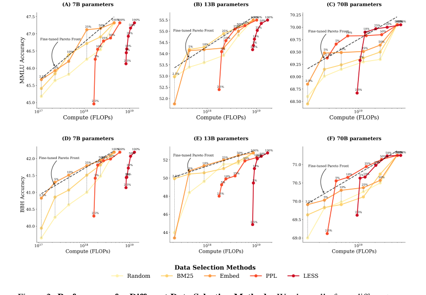 Figure 2. Performance for Different Data Selection Methods. We show all of our different runs for a given model size, where each scatter point is the final target task performance of a single run. (A, B, C) show MMLU results across three model sizes, while (D, E, F) present BBH results across three model sizes. For each run, we determine the optimal finetuning strategy—a combination of data selection method and number of finetuning tokens—that achieves the highest performance un- der a particular FLOPs budget. We fit a pareto front in dashed line based on these optimal strategies, which is a line in the linear-log space. At small and medium compute budgets (A, B, D, E), cheaper data selection methods like BM25 and EMBED outperform PPL and LESS, which rely on model information. At larger compute budgets (C, F), however, PPL and LESS become compute-optimal after using 5% of the fine-tuning tokens
* **Contrast with Fixed Training Budget (Figure 5a)**: The paper provides a crucial counter-example in Figure 5 (a). If you *only* consider the training budget (ignoring selection cost), then LESS consistently *outperforms* all other methods. This stark contrast between Figure 5(a) and Figure 2 is the smoking gun: it definitively shows that *considering the total compute budget (selection + training)* fundamentally changes which data selection strategy is optimal. The paper's core mechanism – the compute-constrained objective – directly leads to different conclusions about method efficacy.
- Extrapolation Results (Figures 9 and 10): These figures provide quantitative evidence for the "tipping point." They show that PPL and LESS do become compute-optimal, but only when the training model is significantly larger than the model used for data selection. Specifically, PPL requires a training-to-selection model size ratio of 5x (around 35B parameters for the training model), and LESS requires a ratio of 10x (around 70B parameters). This mathematically precise finding, derived from their parametric model fitted to empirical data, provides undeniable evidence of the conditions under which these more expensive methods become viable. It's not that they never work, but that their compute cost dictates a specific scale requirement for the training model.
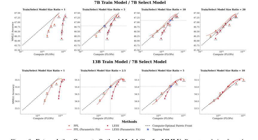 Figure 9. Extrapolating Compute-Optimal Model Size for MMLU. By extrapolating from the parametric fits obtained from the 7B and 13B model results for MMLU, we can find the compute- optimal ratio between the training model size and the selector model size required for the perplexity- based and gradient-based method. For perplexity-based data selection, our extrapolation suggests that training model should be larger (5x) than the selector model—around 35B model parameters. For gradient-based data selection to be compute-optimal, our extrapolation suggest that the training model should be significantly larger (10x) than the selector model—specifically, around 70B param- eters in this case
In essence, the authors didn't just claim that compute costs matter; they meticulously measured them, modeled their impact, and empirically demonstrated that cheaper methods often win the compute-efficiency race, especially for smaller LLMs. The evidence is in the curves and the quantified ratios.
Discussion Topics for Future Development and Evolution
This paper opens up a rich vein of research. Here are some discussion topics, presented from diverse perspectives, to stimulate further critical thinking:
-
Dynamic and Adaptive Data Selection Strategies:
- Current Limitation: The paper evaluates fixed data selection methods.
- Future Direction: Can we develop an intelligent agent that dynamically chooses or combines data selection methods based on the current compute budget, the target LLM size, and the observed performance? For example, start with a cheap method, and if the budget allows and performance gains plateau, switch to a more sophisticated method for a smaller, highly critical subset of data. This would involve real-time monitoring of FLOPs and performance, perhaps using reinforcement learning or adaptive control systems.
- Critical Thinking: How would such an agent handle uncertainty in performance prediction or sudden changes in budget? What are the computational costs of the "agent" itself?
-
Cost-Aware LLM Architectures and Finetuning Methods:
- Current Limitation: Data selection methods are often developed independently of the LLM architecture or finetuning technique.
- Future Direction: Can we design LLMs or finetuning methods (e.g., LoRA variants) that are inherently more amenable to compute-efficient data selection? For instance, could an LLM be designed with "selection-friendly" intermediate representations that make perplexity or gradient calculations significantly cheaper? Or could finetuning methods be developed that are less sensitive to data quality, reducing the need for expensive selection?
- Critical Thinking: Would such specialized architectures compromise generalizability or other performance metrics? What are the trade-offs between selection-friendliness and core model capabilities?
-
Amortization Beyond Multi-Task Settings:
- Current Limitation: The paper touches on multi-task amortization (Figure 4), where selection costs are spread across multiple finetuning runs for different tasks.
- Future Direction: Explore other amortization scenarios. What about continuous learning, where an LLM is periodically updated with new data? Can expensive data selection be performed once and then reused for multiple subsequent finetuning cycles or for different users with similar needs? Consider a "data selection as a service" model where pre-computed utility scores or selected subsets are shared.
- Critical Thinking: How quickly do utility scores become stale in a dynamic data environment? What are the privacy and intellectual property implications of sharing selected datasets or utility scores?
-
Beyond FLOPs: A Holistic Compute Cost Model:
- Current Limitation: The paper primarily focuses on FLOPs as the measure of compute cost.
- Future Direction: Expand the compute cost model to include other critical resources. This could involve:
- Memory Usage: Especially important for large models and resource-constrained environments.
- Energy Consumption: Directly impacts environmental sustainability and operational costs.
- Human-in-the-Loop Costs: For methods that require human labeling or validation, this cost can be substantial.
- Latency: The time taken for selection and training might be a critical factor in real-world deployment.
- Critical Thinking: How do these different cost dimensions interact? Is there a single, unified metric that can capture all these aspects, or do we need multi-objective optimization?
-
Predictive Modeling of $\lambda$ and Optimal Ratios:
- Current Limitation: The efficiency parameter $\lambda$ and the optimal training-to-selection model size ratios are determined empirically by fitting the parametric model.
- Future Direction: Can we develop theoretical frameworks or meta-learning approaches to predict $\lambda$ or the optimal ratios for new tasks, datasets, or model architectures without running extensive empirical sweeps? This would involve understanding the intrinsic properties of data, tasks, and models that influence selection efficiency.
- Critical Thinking: What features of a dataset or task correlate with a higher $\lambda$ for a given selection method? Can we use smaller pilot experiments to inform these predictions for larger-scale deployments?
-
Ethical Implications of Compute-Constrained Selection:
- Current Limitation: The paper focuses on efficiency and performance.
- Future Direction: Consider the ethical implications. If cheaper methods are preferred under compute constraints, do they inadvertently introduce biases or reduce fairness compared to more sophisticated methods that might identify more diverse or representative data? For example, if BM25 selects data based on common keywords, it might reinforce existing biases in the data.
- Critical Thinking: How can we ensure that compute-optimal data selection doesn't lead to "good enough" models that are less robust or fair than those trained with more expensive, but potentially more equitable, data selection? Is there a minimum "quality" threshold for data selection that should be maintained, even if it's not strictly compute-optimal?
These discussion points highlight that while this paper provides a brilliant and practical framework, the journey towards truly optimal and responsible LLM finetuning under real-world constraints is far from over.
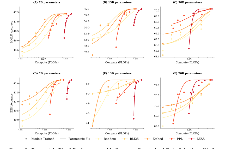 Figure 3. Parametric Fit of Performance with Compute-Constrained Data Selection. We fit a parametric model of the performance in Equation (3) and display that as curves to pair with the empirical results as scatter points. (A, B, C) show MMLU results and their parametric fit across three model sizes, while (D, E, F) present BBH results and their parametric fit across three model sizes