LiteTracker: Leveraging Temporal Causality for Accurate Low-latency Tissue Tracking

Background & Academic Lineage

The problem of tracking tissue in endoscopic video streams originates from the need for surgical navigation and extended reality (XR) systems to maintain a stable reference on deformable, non-rigid biological surfaces. Historically, this field evolved from general computer vision "point tracking" (like the classic Particle Videos approach) into specialized medical applications where the primary challenge is the high-stakes requirement for both extreme accuracy and ultra-low latency.

The fundamental "pain point" of previous state-of-the-art models, such as CoTracker3, is their reliance on sliding-window processing. These models require the accumulation of multiple frames (a "window") before they can output a prediction. In a surgical setting, this creates a significant, artificial delay—often exceeding 200ms—which is unacceptable for real-time robotic feedback or augmented reality overlays. Furthermore, the iterative refinement modules in these models are computationally expensive, leading to a linear increase in runtime that prevents high-speed, frame-by-frame tracking.

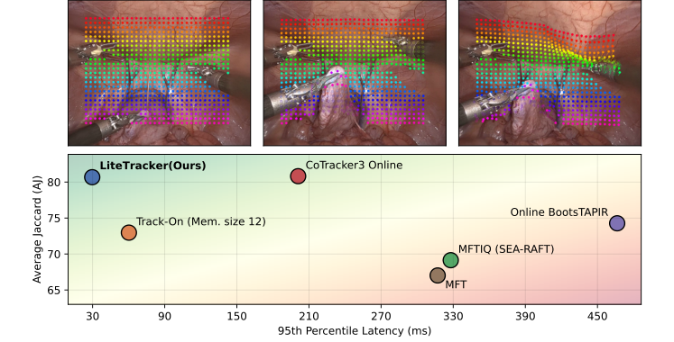Figure 1. (Top) Demonstration of LiteTracker on a video from STIR Challenge 2024 dataset [16]. (Bottom) Latency and tracking accuracy comparison. Average Jaccard (AJ) metric is computed on SuPer dataset [11]. Latencies showcase the 95th percentile of inference step measurements for 1,024 points initalized at the first frame of a video with 615 frames. LiteTracker is approximately 2× faster than the fastest evaluated method, Track-On [1], and 7× than its predecessor, CoTracker3 [9], while exhibiting close to state-of-the-art tracking accuracy

Intuitive Domain Terms

• Sliding-Window Processing: Imagine trying to understand a conversation by waiting for a person to finish an entire 16-word sentence before you are allowed to process any of the words. You are always 16 words behind. LiteTracker changes this to a "live" stream, where you process each word as it is spoken.
• Temporal Memory Buffer: Think of this as a "short-term memory" notebook. Instead of re-calculating complex math from scratch for every new frame, the system writes down the important results from previous frames in a notebook (the buffer) and just looks them up when needed, saving massive amounts of time.
• Exponential Moving Average (EMA) Flow: This is like predicting where a car will be based on its recent speed and direction. Instead of guessing randomly, you use a weighted average of its past movements to make a very smart, quick guess about where it will be in the next instant, avoiding the need for slow, repeated corrections.
• Non-rigid Deformations: Unlike a rigid object (like a table), tissue stretches, folds, and squishes. Tracking it is like trying to track a specific spot on a piece of fabric that is being constantly pulled and twisted by surgical tools.

Notation Table

Notation	Description
$I_t$	The video frame at time $t$
$Q$	The set of query points to be tracked
$V_t$	Predicted visibility score at time $t$ ($V_t \in [0, 1]$)
$C_t$	Predicted confidence score at time $t$ ($C_t \in [0, 1]$)
$P_t$	Predicted 2D location $(x, y)$ of a point at time $t$
$T_W$	Window size (number of frames processed together)
$S$	Stride (number of frames skipped between processing)
$T_B$	Capacity of the temporal memory buffer
$F_t$	Exponential moving average flow vector
$\alpha$	Temporal smoothing factor for EMA flow

The authors solved the latency problem by replacing the heavy sliding-window architecture with a frame-by-frame approach supported by a temporal memory buffer. To maintain accuracy without the original iterative refinement, they introduced a smart initialization strategy.

The core of their initialization is the EMA flow, defined as:
$$F_t = \alpha(P_{t-1} - P_{t-2}) + (1 - \alpha)F_{t-1}$$
This equation calculates a motion vector $F_t$ by blending the most recent movement $(P_{t-1} - P_{t-2})$ with the historical trend $F_{t-1}$. By setting $\alpha = 0.8$, the model gives more weight to the most recent motion, allowing it to predict the next location $P_t^{\text{init}}$ with high precision:
$$P_t^{\text{init}} = P_{t-1} + F_t$$
By providing this accurate starting point, the model achieves convergence in a single pass ($L=1$), effectively eliminating the need for the computationally expensive iterative loops that plagued previous models. The temporal memory buffer then ensures that the "heavy lifting" of feature extraction is not repeated, as the system simply retrieves cached correlation features from the ring buffer.

Problem Definition & Constraints

Core Problem Formulation & The Dilemma

The Starting Point and Goal State
The input to the system is a continuous endoscopic video stream, where the goal is to perform "long-term point tracking"—essentially, following specific anatomical landmarks or tissue points across many frames. The desired output is the precise coordinate $(x_t, y_t)$ of these points, along with their visibility and confidence scores, in real-time. The missing link is the ability to maintain high tracking accuracy (which usually requires heavy, multi-frame context processing) while simultaneously meeting the strict, low-latency requirements of an operating room environment.

The Fundamental Dilemma
The authors face a classic trade-off between temporal context and computational latency. To track tissue accurately through complex surgical scenes—characterized by non-rigid deformations, tool occlusions, and rapid camera movements—modern models (like the predecessor, CoTracker3) rely on "sliding-window" processing. This means the algorithm must buffer a sequence of frames (e.g., 16 frames) and perform multiple iterative refinement steps to converge on an accurate position. This creates a "waiting" period that is unacceptable for real-time surgical robotics or XR applications, where every millisecond of delay can lead to desynchronization between the digital overlay and the physical tissue.

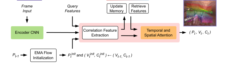Figure 2. LiteTracker’s architecture. Given a video stream and a set of query points, we extract feature maps for each new frame and compute correlation features between the queries and points initialized with exponential moving average flow (EMA flow). We store these correlation features in a temporal memory buffer for efficient re-use on subsequent frames. Utilizing a transformer we propagate spatio-temporal information via attention mechanism to yield new point locations, visibility and confidence scores

To bridge the gap, the authors introduced two primary "training-free" optimizations that bypass the need for heavy, redundant computations.

1. Temporal Memory Buffer (Efficient Feature Reuse)
Instead of re-processing the entire sliding window for every new frame, the authors implemented a ring buffer with a capacity $T_B = 16$. This buffer caches the "correlation features"—the most computationally expensive part of the pipeline involving pair-wise similarity measurements. By storing these, the system avoids redundant calculations, allowing for frame-by-frame processing rather than waiting for a full window stride.

2. Exponential Moving Average (EMA) Flow Initialization
To eliminate the need for multiple iterative refinement steps (which were previously required to "find" the point), the authors introduced a clever initialization strategy. They use an EMA flow, $F_t$, to predict where the point will be before the refinement module even touches it:
$$F_t = \alpha(P_{t-1} - P_{t-2}) + (1 - \alpha)F_{t-1}$$
Where $P_t$ is the point location and $\alpha$ is a smoothing factor (empirically set to $0.8$). This allows the model to calculate the initial location for the new frame as:
$$P^{\text{init}}_t = P_{t-1} + F_t$$
By providing this highly accurate "guess" to the transformer, the model can achieve convergence in a single pass ($L := 1$) through the refinement module. This effectively collapses the computational cost of the iterative loop, which is a major breakthrough in reducing latency.

Why This Approach

The Inevitability of the Choice

The authors of LiteTracker identified a fundamental bottleneck in modern surgical tracking: the trade-off between the high accuracy of transformer-based long-term point trackers (like CoTracker3) and the strict, low-latency requirements of real-time operating room environments. Traditional "SOTA" methods, while robust, rely on sliding-window processing that forces the system to wait for a buffer of frames (e.g., 16 frames) before producing an output. This introduces significant "implicit latency," which is unacceptable for surgical robotics where even a few hundred milliseconds of delay can compromise safety.

Comparative Superiority

LiteTracker is qualitatively superior because it shifts the paradigm from window-based batch processing to a frame-by-frame approach without sacrificing the temporal context that makes transformer models effective.
- Structural Advantage: By implementing a temporal memory buffer (a ring buffer with capacity $T_B = 16$), the authors avoid the redundant re-computation of expensive correlation features. This reduces the computational overhead from $O(N \cdot T_W)$ to a more efficient per-frame update, where $N$ is the number of points and $T_W$ is the window size.
- Efficiency: The method achieves an inference latency of $29.67$ ms, which is approximately $7\times$ faster than CoTracker3 and $2\times$ faster than the previous fastest method, Track-On. When accounting for the implicit delay of sliding-window accumulation, the total latency improvement over CoTracker3 is roughly $16.6\times$.

Mathematical & Logical Mechanism

The Mathematical Engine: Exponential Moving Average (EMA) Flow

The core mathematical innovation that allows LiteTracker to achieve high-speed, low-latency performance without the need for computationally expensive iterative refinement is the Exponential Moving Average (EMA) Flow initialization.

The master equation governing this mechanism is:

$$F_t = \alpha(P_{t-1} - P_{t-2}) + (1 - \alpha)F_{t-1}$$

Tearing Down the Equation

• $F_t$: This is the predicted motion vector (flow) for the current frame $t$. It represents the displacement of a point from its position at $t-1$ to its estimated position at $t$.
• $\alpha$: This is the temporal smoothing factor (set to $0.8$). It acts as a "memory weight," determining how much the model trusts the most recent observed motion versus the historical trend.
• $(P_{t-1} - P_{t-2})$: This term calculates the instantaneous velocity of the point between the two previous frames. It provides the "current" direction of the tissue.
• $F_{t-1}$: This is the previously computed flow vector. By including this, the author ensures the model maintains a consistent trajectory, acting like a momentum term in physics that prevents the tracking from jittering due to noise.

Results, Limitations & Conclusion

The authors of LiteTracker solved the latency problem by transforming a heavy, iterative, window-based process into a streamlined, single-pass, frame-by-frame process. They achieved this by caching expensive features in a ring buffer and using a simple, elegant mathematical heuristic (EMA flow) to initialize point locations.

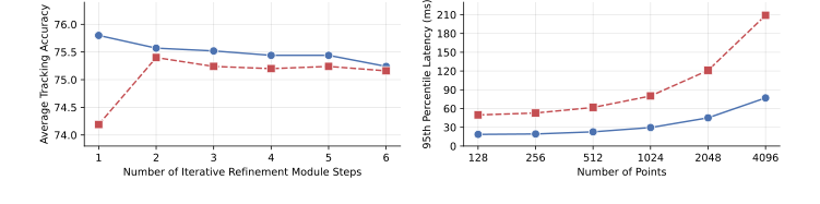Figure 4. Ablation studies. (Left) Exponential moving average flow (EMA flow) initial- ization improves tracking convergence, leading to its highest average tracking accuracy on the STIR Challenge 2024 dataset [16] with a single pass through the iterative refine- ment module. (Right) Temporal memory buffer improves runtime efficiency by approx- imately 2.7 times and provides low-latency inference during frame-by-frame tracking

Experimental Validation

The authors ruthlessly tested their architecture against baseline models like CoTracker3, Track-On, and various MFT variants. The evidence is compelling:
* Speed: LiteTracker achieved an inference latency of 29.67 ms, making it approximately 7 times faster than CoTracker3 and 2 times faster than the previous fastest method, Track-On.
* Accuracy: Despite the massive speedup, it maintained competitive tracking accuracy on the STIR and SuPer datasets.
* Ablation Studies: The authors proved that their EMA flow initialization actually degrades performance if too many refinement steps are used, confirming that their initialization is so precise that further iterations are not only unnecessary but detrimental.