Hybrid Boundary Physics-Informed Neural Networks for Solving Navier-Stokes Equations with Complex Boundary
Physics-informed neural networks (PINN) have achieved notable success in solving partial differential equations (PDE), yet solving the Navier-Stokes equations (NSE) with complex boundary conditions remains a...
Background & Academic Lineage
To understand the precise origin of the problem addressed in this paper, we have to look at the intersection of fluid mechanics and modern artificial intelligence. For decades, scientists and engineers have relied on the Navier-Stokes equations (NSE) to describe the dynamic behavior of viscous fluids—essentially, how liquids and gases move. Traditionally, these highly complex, nonlinear equations were solved using Computational Fluid Dynamics (CFD). However, CFD requires a process called "mesh generation," where the physical space is divided into a massive grid of tiny shapes. Creating this mesh for complex, irregular shapes is incredibly difficult, time-consuming, and can lead to numerical instability.
In 2019, a breakthrough occurred: Physics-Informed Neural Networks (PINNs) were introduced. PINNs use deep learning to solve these equations without needing a mesh at all. They do this by embedding the physical laws directly into the neural network's learning process. However, as researchers began applying PINNs to real-world fluid problems, a new, highly specific problem emerged: dealing with complex boundaries (like fluid flowing around irregular obstacles).
The fudamental limitation—or "pain point"—of previous PINN approaches is what researchers call the "loss conflict problem." In a conventional PINN, the AI is asked to learn the physical rules of the fluid (the PDE loss) and the rules of the physical boundaries (the boundary condition loss) simultanously. Because both of these goals are thrown into a single mathematical bucket (the loss function), the network often struggles to balance them. When the geometric boundaries get highly complex, the network gets confused. It might satisfy the fluid dynamics perfectly but fail to respect the solid walls, or vice versa. Previous attempts to fix this by forcing "hard constraints" using analytical math resulted in distorted, erratic predictions near complex junctions because those mathematical functions weren't natural. The authors wrote this paper to decouple these conflicting goals, creating a hybrid system that handles the boundaries and the internal fluid physics separately but cooperatively.
Here are a few highly specialized domain terms from the paper, translated into intuitive analogies for a complete beginner:
- Navier-Stokes Equations (NSE):
- Analogy: Think of these as the ultimate, unbreakable "traffic laws" for water and air molecules. Just as traffic laws dictate who yields, how fast you can go, and how to navigate an intersection without crashing, the NSE dictate exactly how fluid molecules must flow, swirl, and interact with pressure and friction without violating the laws of physics.
- Physics-Informed Neural Networks (PINN):
- Analogy: Imagine teaching a student to paint a realistic landscape. A standard neural network just memorizes millions of photos and tries to copy the pixel patterns. A PINN, however, is a student who is also taught the actual laws of gravity and light perspective. Because they know the underlying rules, they will never accidentally paint a waterfall flowing upwards, even if they've never seen that specific waterfall before.
- Loss Conflict Problem:
- Analogy: Imagine you are hiring a chef and giving them two strict instructions: "Make the dish incredibly spicy" and "Make sure it is completely mild for children." The chef becomes paralyzed trying to optimize for two completely contradictory demands at the same time, resulting in a terrible meal. In PINNs, the network gets similarly paralyzed trying to perfectly satisfy the internal fluid physics and the complex boundary rules at the exact same time.
- Distance Metric Network ($\mathcal{N_D}$):
- Analogy: Think of this as the parking proximity sensor on a modern car. As you back up, it beeps faster the closer you get to a wall. This specific sub-network acts as a spatial sensor, telling the main AI exactly how close it is to a boundary, so the AI knows exactly when to start paying strict attention to the "wall rules" versus the "open water rules."
Below is a table organizing the key mathematical notations, variables, and paramters necessary for understanding the mechanics of the proposed HB-PINN model:
| Notation | Type | Description |
|---|---|---|
| $\mathbf{u}$ | Variable | The velocity vector of the fluid (comprising horizontal and vertical components $u$ and $v$). |
| $p$ | Variable | The fluid pressure at a given point in space and time. |
| $\rho$ | Parameter | The density of the fluid (remains constant for incompressible flows). |
| $\nu$ | Parameter | The dynamic viscosity coefficient, representing the fluid's internal friction or "thickness." |
| $q(\mathbf{x}, t)$ | Variable | A general placeholder for any physical quantity of interest being predicted (e.g., velocity or pressure) at spatial coordinates $\mathbf{x}$ and time $t$. |
| $\mathcal{P}_q(\mathbf{x}, t)$ | Function | The output of the Particular Solution Network ($\mathcal{N_P}$), which is strictly trained to satisfy the boundary conditions. |
| $\mathcal{D}_q(\mathbf{x}, t)$ | Function | The output of the Distance Metric Network ($\mathcal{N_D}$), representing the spatial distance from a point to the nearest boundary. |
| $\mathcal{H}_q(\mathbf{x}, t)$ | Function | The output of the Primary Network ($\mathcal{N_H}$), which focuses purely on solving the internal fluid dynamics (the governing PDE). |
| $\mathcal{L}$ | Parameter | The loss function, representing the error the network is trying to minimize. It is split into parts like $\mathcal{L}_{PDE}$ (equation error) and $\mathcal{L}_{BC}$ (boundary error). |
| $\lambda_i$ | Parameter | Weighting coefficients used to tell the network which part of the loss function is more important to focus on during training. |
| $\alpha$ | Parameter | A positive value controlling the growth rate (steepness) of the distance function, determining how sharply the network transitions from boundary rules to interior rules. |
Problem Definition & Constraints
Imagine trying to predict exactly how water flows around a jagged rock or through a complex system of pipes. Traditionally, engineers use Computational Fluid Dynamics (CFD), which requires drawing a microscopic, perfect grid over the entire fluid area—a process called mesh generation that is notoriously tedious and prone to numerical instability.
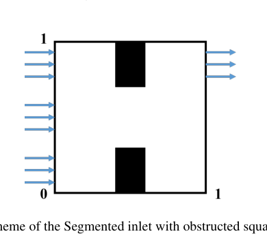 Figure 12. Scheme of the Segmented inlet with obstructed square cavity flow
Physics-Informed Neural Networks (PINNs) promised a brilliant shortcut: skip the grid entirely and just teach a neural network the laws of physics. However, when applied to real-world, complex shapes, these networks hit a massive mathematical wall. Let's break down exactly why this happens and the specific problem this paper attempts to solve.
The Starting Point and The Goal State
The Input (Current State):
We start with a set of spatiotemporal coordinates $(x, t)$ and the governing rules of fluid dynamics, known as the incompressible Navier-Stokes equations (NSE):
$$ \nabla \cdot \mathbf{u} = 0 $$
$$ \frac{\partial \mathbf{u}}{\partial t} + (\mathbf{u} \cdot \nabla)\mathbf{u} + \frac{1}{\rho}\nabla p - \nu \nabla^2 \mathbf{u} = 0 $$
Alongside these equations, we have highly complex boundary conditions—such as segmented inlets or irregular obstructing structures where the fluid velocity must be exactly zero (the no-slip condition).
The Output (Goal State):
The desired endpoint is a trained neural network that can instantly and accurately output the velocity vector $\mathbf{u}$ (composed of $u$ and $v$) and the fluid pressure $p$ at any given point.
The Mathematical Gap:
The missing link is a reliable mathematical bridge that forces a continuous neural network to strictly obey the sharp, irregular rules at the boundaries without destroying its ability to calculate the smooth, continuous physics happening inside the fluid.
The Painful Dilemma
Previous reasearchers have been trapped in a brutal trade-off known as the "loss conflict problem." When trying to solve this, improving one aspect fundamentally breaks another:
- The Soft Constraint Trap: In conventional PINNs, you tell the network to minimize a single, giant loss function that includes both the physics errors (PDE loss) and the boundary errors. But the network gets overwhelmed. It tries to minimize both simultanously, but the complex boundaries generate wild mathematical gradients that actively fight against the physics gradients during training. The network ends up compromising, resulting in inaccurate boundaries that pollute the entire fluid simulation.
- The Hard Constraint Trap: To fix this, scientists tried "hard-constrained" PINNs (like hPINN). They mathematically forced the network's output to be exactly zero at the boundaries using an analytical distance function. Here is the painful dilemma: for complex geometries, these exact mathematical formulas are highly unnatural. Forcing the network through these rigid mathematical hoops causes the internal fluid predictions to become distorted, erratic, and discontinuous. You perfectly fix the boundary, but you completely break the fluid dynamics inside.
The Harsh Walls and Constraints
What makes this problem insanely difficult to solve? The authors ran into several harsh, realistic walls:
- Geometrical Infeasibility: To make hard constraints work, you need a distance function, $D_q(x, t)$, which calculates the exact distance from any point to the boundary. For a simple flat wall, this is a basic algebra equation. For complex, segmented, or irregular boundaries, deriving an exact analytical expression is mathematically impossible.
- Extreme Gradient Pathologies: To force a standard network to pay attention to the boundaries, researchers have to artificially inflate the boundary loss weights (e.g., setting the boundary weight $\lambda_2 = 1000$ while the physics weight $\lambda_1 = 1$). This creates a massive imbalance. The network becomes hyper-focused on memorizing the edges and completely ignores the actual governing equations of the fluid.
- Highly Nonlinear Physics: The Navier-Stokes equations are notoriously unforgiving because of the nonlinear convective acceleration term, mathematically represented as $(\mathbf{u} \cdot \nabla)\mathbf{u}$. Because of this nonlinearity, even a microscopic error at a complex boundary will rapidly amplify, destabilizing the entire flow field prediction.
- Network Capacity Limits: Asking a single neural architecure to simultaneously learn the sharp, high-frequency transitions required at a complex boundary and the smooth, low-frequency physical dynamics of the interior fluid simply exceeds standard optimization capabilities. The network's weights cannot easily represent both behaviors at once.
Why This Approach
To truly understand why the authors built the Hybrid Boundary Physics-Informed Neural Network (HB-PINN), we first need to step into their shoes and look at the fundamental nature of the problem they were trying to solve: modeling fluid dynamics using the Navier-Stokes equations (NSE).
If you are wondering why the authors didn't just throw a popular, trendy model like a GAN, a Transformer, or a Diffusion model at this, the answer lies in the strict constraints of physics. We aren't trying to generate plausible-looking pictures of water or predict the next word in a sequence. We need to deterministically solve highly non-linear partial differential equations (PDEs). Generative models map noise to data distributions, which is practically useless when you need strict, mathematical adherence to physical conservation laws (like mass and momentum).
Because traditional deep learning fails here, the scientific community relies on Physics-Informed Neural Networks (PINNs). PINNs embed the actual physics equations into the neural network's loss function. However, the authors hit a massive roadblock—the exact moment they realized the current "SOTA" PINNs were fundamentally broken for real-world applications.
The problem arises when fluid flows around complex obstacles (like a blocked cavity or a segmented inlet). Conventional PINNs (often called soft-constrained PINNs, or sPINNs) try to learn the governing physics equations and the boundary conditions simultanously by cramming them into a single, massive loss function. This creates a severe "loss conflict." The gradients from the boundary conditions and the gradients from the interior physics literally fight each other during backpropagation. The network gets confused, and accuracy plummets.
Previous attempts to fix this involved hard-constrained PINNs (hPINNs), which force the network to respect boundaries using exact, analytical mathematical formulas. But as the authors explicitly demonstrate in Appendix D of the paper, when you have complex, irregular geometries, these analytical functions break down. They become non-natural and cause highly distorted, discontinuous, and erratic outputs inside the fluid domain.
Faced with this dilemma—soft constraints cause gradient conflicts, and hard constraints mathematically break down on complex shapes—the authors realized that a decoupled, composite architecutre was the only viable solution.
They designed HB-PINN to divide and conquer the problem using three distinct subnetworks:
1. $\mathcal{N_P}$ (Particular Solution Network): A network trained solely to satisfy the boundary conditions.
2. $\mathcal{N_D}$ (Distance Metric Network): A network that learns the spatial distance from any point to the boundaries.
3. $\mathcal{N_H}$ (Primary Network): The main network dedicated entirely to solving the governing PDE in the interior.
They married these networks together using a brilliant composite formulation for any physical quantity $q$ (like velocity or pressure):
$$N_q(\mathbf{x}, t) = \mathcal{N}_{\mathcal{P}_q}(\mathbf{x}, t) + \mathcal{N}_{\mathcal{D}_q}(\mathbf{x}, t) \cdot \mathcal{N}_{\mathcal{H}_u}(\mathbf{x}, t)$$
Here is why this specific mathematical model is qualitatively superior to the previous gold standard. By pre-training $\mathcal{N_P}$ and $\mathcal{N_D}$ and then freezing their weights, the distance function $\mathcal{N_D}$ acts as a spatial gatekeeper. At the exact boundary, $\mathcal{N_D}$ equals 0, meaning the main network $\mathcal{N_H}$ is completely zeroed out, and the output relies 100% on the boundary network $\mathcal{N_P}$. As you move away from the boundary into the fluid, $\mathcal{N_D}$ smoothly transitions to 1, allowing the main network $\mathcal{N_H}$ to take over and solve the physics.
To ensure this transition is perfectly smooth and doesn't destabilize the network, they introduced a power-law function to refine the distance metric:
$$f(\hat{\mathcal{D}}_q) = 1 - (1 - \hat{\mathcal{D}}_q / \max(\hat{\mathcal{D}}_q))^\alpha$$
By tuning the parameter $\alpha$, they can control exactly how steeply the network transitions from the boundary to the interior.
While the paper does not explicitly claim a memory complexity reduction from $O(N^2)$ to $O(N)$ (to be honest, the computational bottleneck here is optimization, not just memory scaling), it demonstrates a structural advantage that makes it overwhelmingly superior: the complete elimination of gradient pathology. Because the primary network $\mathcal{N_H}$ no longer has to worry about satisfying the boundaries, it can focus exclusively on minimizing the PDE residual. This structural decoupling results in an order-of-magnitude reduction in Mean Squared Error (MSE) compared to SOTA models like XPINN, SA-PINN, and PirateNet.
This appraoch represents a perfect "marriage" between the problem's harsh requirements and the solution's unique properties. The problem demanded strict boundary enforcement without relying on impossible analytical math; the solution provided it by using a neural network ($\mathcal{N_D}$) to approximate the geometry, effectively turning a geometrically impossible hard constraint into a highly flexible, learnable one.
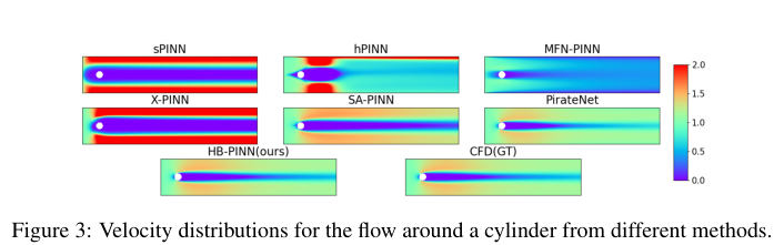 Figure 3. Velocity distributions for the flow around a cylinder from different methods
Mathematical & Logical Mechanism
To understand the breakthrough presented in this paper, we must first look at the fundemental problem of simulating fluids. For decades, engineers have relied on Computational Fluid Dynamics (CFD) to understand how air flows over a wing or water moves through a pipe. These traditional methods require "meshing"—chopping the space into millions of tiny geometric grids. Meshing is computationally expensive, tedious, and prone to instability when the boundaries (like the shape of an obstacle) become highly complex.
Recently, Physics-Informed Neural Networks (PINNs) emerged as a revolutionary alternative. Instead of using a mesh, PINNs use deep learning to guess the solution, penalizing the neural network if its guess violates the laws of physics (specifically, the Navier-Stokes equations). However, standard PINNs hit a massive roadblock: the "loss conflict." When a fluid hits a complex boundary, the neural network gets confused. It tries to simultaneously satisfy the complex boundary conditions (the walls) and the fluid dynamics (the interior). The mathematical gradients fighting over these two objectives end up canceling each other out, leading to highly inaccurate simulations.
The authors of this paper solved this by creating the Hybrid Boundary PINN (HB-PINN). Instead of forcing one network to learn everything, they built a composite architecure that strictly separates the boundary constraints from the interior physics.
Here is the absolute core equation that powers this entire framework:
$$ \mathcal{N}_q(\mathbf{x}, t) = \mathcal{N}_{\mathcal{P}_q}(\mathbf{x}, t) + \mathcal{N}_{\mathcal{D}_q}(\mathbf{x}, t) \cdot \mathcal{N}_{\mathcal{H}_q}(\mathbf{x}, t) $$
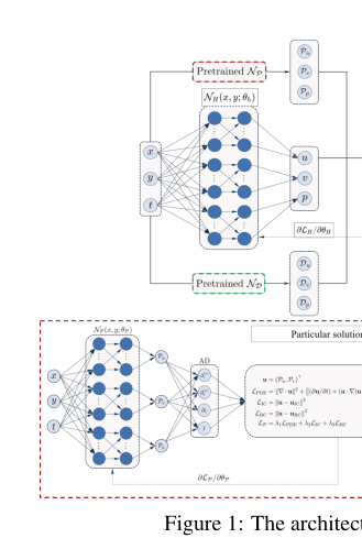 Figure 1. The architecture of the proposed method
Let us tear this equation apart piece by piece to understand exactly how it manipulates the data.
- $\mathcal{N}_q(\mathbf{x}, t)$:
- Mathematical Definition: The final composite output function for a specific physical quantity $q$ (which could be velocity $u$, velocity $v$, or pressure $p$) at a given spatial coordinate $\mathbf{x}$ and time $t$.
- Physical/Logical Role: This is the finished product. It represents the exact state of the fluid at any given point in space and time.
- $\mathcal{N}_{\mathcal{P}_q}(\mathbf{x}, t)$:
- Mathematical Definition: The output of the Particular Solution Network.
- Physical/Logical Role: This acts as the "boundary enforcer." It is a pre-trained neural network whose sole job is to perfectly memorize and satisfy the boundary conditions (e.g., ensuring velocity is exactly zero at a solid wall).
- $+$ (Addition Operator):
- Why addition instead of multiplication? Addition allows for the principle of superposition. The network uses $\mathcal{N}_{\mathcal{P}_q}$ as a foundational baseline. If the authors had used multiplication here, a zero value from the boundary network would act like a black hole, completely annihilating any physics calculated in the interior. Addition allows the model to say: "Start with this boundary baseline, and add the interior fluid dynamics on top of it."
- $\mathcal{N}_{\mathcal{D}_q}(\mathbf{x}, t)$:
- Mathematical Definition: The output of the Distance Metric Network, shaped by a power-law function.
- Physical/Logical Role: This is a spatial mask or a "volume knob." It outputs a value of exactly $0$ at the boundaries and rapidly scales up to $1$ as you move into the interior of the fluid.
- $\cdot$ (Multiplication Operator):
- Why multiplication instead of addition? This acts as a spatial mutliplier or a gating mechanism. By multiplying the distance metric with the primary physics network, the equation forces the physics network to be multiplied by $0$ at the boundaries. This completely mutes the interior physics engine at the walls, ensuring that the boundary enforcer ($\mathcal{N}_{\mathcal{P}_q}$) has 100% absolute authority at the edges.
- $\mathcal{N}_{\mathcal{H}_q}(\mathbf{x}, t)$:
- Mathematical Definition: The output of the Primary Network.
- Physical/Logical Role: This is the heavy-lifting physics engine. It is a large neural network dedicated entirely to solving the Navier-Stokes equations in the interior of the domain.
Step-by-step Flow
Imagine a single abstract data point—a coordinate in space and time, $(\mathbf{x}, t)$—entering this mathematical assembly line.
First, the coordinate is duplicated and fed into three separate neural networks simultaneously. In the first path, the Particular Solution Network evaluates the point and outputs a baseline physical value that perfectly respects the nearest wall. In the second path, the Distance Metric Network measures how far this point is from the boundary, outputting a percentage (e.g., $0.0$ if it's on the wall, $0.99$ if it's deep inside the fluid). In the third path, the Primary Network calculates the complex fluid dynamics for that point.
Next, the assembly line merges. The raw physics calculation from the Primary Network is multiplied by the distance percentage. If the point is on a wall, the physics calculation is multiplied by zero and discarded. If it is in the open fluid, it is kept almost entirely intact. Finally, this scaled physics calculation is added to the baseline boundary value. The result is a seamless, physically accurate prediction that perfectly respects complex geometries without the networks fighting each other.
Optimization Dynamics
To understand how this mechanism actually learns, we have to look at how the loss landscape is shaped. In a standard PINN, the loss function is a messy combination of boundary errors and physics errors. The gradients (the mathematical arrows pointing the network toward the correct answer) constantly collide.
The HB-PINN solves this through a staged optimization dynamic. First, the boundary network ($\mathcal{N}_{\mathcal{P}}$) and the distance network ($\mathcal{N}_{\mathcal{D}}$) are pre-trained and then frozen. Their weights are locked in place.
Because the boundaries are already perfectly handled and locked, the Primary Network ($\mathcal{N}_{\mathcal{H}}$) is optimized using only the physics loss:
$$ \mathcal{L}_{\mathcal{H}} = \frac{1}{N_{\text{PDE}}} \sum_{i=1}^{N_{\text{PDE}}} \left( \| \nabla \cdot \mathbf{\hat{u}} \|^2 + \left\| \frac{\partial \mathbf{\hat{u}}}{\partial t} + (\mathbf{\hat{u}} \cdot \nabla)\mathbf{\hat{u}} + \frac{1}{\rho}\nabla \hat{p} - \nu\nabla^2\mathbf{\hat{u}} \right\|^2 \right) $$
Here, the authors use a summation ($\sum$) over $N_{\text{PDE}}$ discrete collocation points rather than a continuous spatial integral. Why? Because neural networks learn through discrete batches of data. We cannot compute a true continuous integral over an infinite number of points in a computer's memory, so we sample thousands of discrete points and sum their errors to approximate the integral.
The terms inside the norms ($\| ... \|^2$) are the exact residuals of the incompressible Navier-Stokes equations (mass conservation and momentum conservation). Because the boundary constraints are mathematically guaranteed by the frozen subnetworks, the loss landscape for $\mathcal{L}_{\mathcal{H}}$ is dramatically smoothed out. The gradients no longer suffer from pathological conflicts. They point strictly downhill toward minimizing the physics residual. The network converges faster, avoids local minima caused by geometric complexities, and achieves state-of-the-art accuracy by simply allowing the physics engine to focus 100% of its learning capacity on the fluid dynamics.
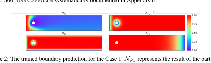 Figure 2. The trained boundary prediction for the Case 1. NPu represents the result of the particular solution network for u, while NDu, NDv, and NDp respectively represent the results of the distance metric network for u, v, and p
Results, Limitations & Conclusion
The Background: Rules of the River and the AI that Learns Them
To understand this paper, we first need to understand two concepts: the Navier-Stokes Equations (NSE) and Physics-Informed Neural Networks (PINNs).
Imagine you are trying to predict exactly how water will flow around a rock in a river. In physics, we use the Navier-Stokes Equations, which are essentially the fundamental laws of motion for liquids and gases. They calculate how pressure, velocity, and viscosity interact. However, these equations are notoriously difficult to solve. Traditionally, engineers use Computational Fluid Dynamics (CFD), which involves chopping the river into millions of tiny digital grids (mesh generation) and calculating the math for each grid. It is highly accurate but incredibly slow and computationally expensive.
Enter PINNs. Instead of chopping up the space into a grid, we ask an Artificial Intelligence (a neural network) to guess the flow of the water. But we don't just let it guess blindly; we embed the Navier-Stokes equations directly into the AI's "loss function" (its penalty system). If the AI guesses a flow that violates the laws of physics, it gets penalized. Over time, it learns to predict physically accurate fluid dynamics without needing a complex grid.
However, there is a catch: Boundary Conditions (BCs). The rules of the river change at the boundaries. For example, water touching the surface of the rock has a velocity of exactly zero (this is called the no-slip condition).
The Motivation and the Constraint: The "Loss Conflict"
The core problem this paper tackles is that standard PINNs are terrible at multitasking.
When a standard PINN tries to solve a fluid problem, it has to minimize two penalties simultaneously:
1. The PDE Loss: "Am I obeying the physics of the water flowing in the middle of the river?"
2. The BC Loss: "Am I obeying the rule that water stops moving exactly at the rock's surface?"
When the boundaries are simple (like a straight pipe), the AI handles this fine. But when the boundaries are complex—like multiple jagged rocks or segmented inlets—the AI suffers from a loss conflict. The gradients (the mathematical nudges telling the AI how to improve) for the boundary rules and the interior physics start fighting each other. The AI gets confused, compromises, and ends up failing at both.
The constraint the authors had to overcome was finding a way to strictly enforce the boundary rules without disrupting the AI's ability to learn the physics in the interior domain, all while keeping the math smooth and differentiable so the neural network could actually process it.
The authors solved this by completely decoupling the problem. Instead of forcing one AI to do everything, they created a Hybrid Boundary PINN (HB-PINN) that uses three specialized subnetworks.
Mathematically, they redefined the prediction of any physical quantity $q(x, t)$ (like velocity or pressure) using this beautiful composite equation:
$$q(x, t) = \mathcal{N}_{P_q}(x, t) + \mathcal{N}_{D_q}(x, t) \cdot \mathcal{N}_{H_q}(x, t)$$
Let's break down exactly what this means:
- $\mathcal{N}_{P_q}$ (The Particular Solution Network): This network is pre-trained with one primary job: satisfy the boundary conditions. It learns what the fluid should be doing right at the walls.
- $\mathcal{N}_{D_q}$ (The Distance Metric Network): This is the clever part. It calculates how far a point is from the boundary. It outputs exactly $0$ at the boundary and rapidly increases to $1$ as you move into the open fluid. They used a specific power-law function to control this transition:
$$f(\hat{D}_q) = 1 - (1 - \hat{D}_q / \max(\hat{D}_q))^\alpha$$ - $\mathcal{N}_{H_q}$ (The Primary Network): This network focuses only on the Navier-Stokes equations in the interior of the fluid.
Look at the main equation again. At the boundary, the distance network $\mathcal{N}_{D_q}$ outputs $0$. This means $0 \cdot \mathcal{N}_{H_q}$ becomes $0$, and the interior network is completely silneced. The final answer is just $\mathcal{N}_{P_q}$, which perfectly satisfies the boundary rules! As you move away from the wall, $\mathcal{N}_{D_q}$ becomes $1$, allowing the primary network $\mathcal{N}_{H_q}$ to take over and solve the physics. The loss conflict is mathematically annihilated.
The Experimental Architecure and the "Victims"
The authors didn't just throw a few numbers on a table to claim victory; they engineered a ruthless testing ground. They set up three fluid dynamics scenarios, culminating in a highly complex "segmented inlet with an obstructed square cavity" (essentially a box with multiple blocked entryways and internal walls) under both steady and transient (time-changing) conditions.
The "victims" in this experiment were a who's-who of state-of-the-art physics AI:
* sPINN (The standard baseline)
* hPINN (Hard-constrained PINN, a previous attempt at fixing boundaries)
* MFN-PINN (Modified Fourier Network)
* XPINN & SA-PINN (Advanced domain-decomposition and self-adaptive models)
* PirateNet (A very recent, highly robust architecture)
The Definitive Evidence:
The undeniable proof of HB-PINN's superiority wasn't just in the Mean Squared Error (MSE) tables—though achieving an order-of-magnitude reduction in error is impressive. The definitive evidence was in the visual residual maps.
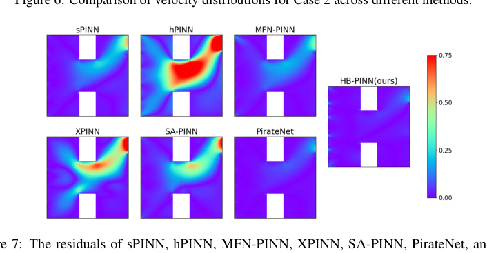 Figure 7. The residuals of sPINN, hPINN, MFN-PINN, XPINN, SA-PINN, PirateNet, and our HB-PINN compared to the GT in Case 2
The authors used high-fidelity Computational Fluid Dynamics (CFD) as the absolute ground truth. When looking at the heatmaps of the errors (residuals), the victim models showed massive, glaring red zones (high error) clustered exactly around the corners of the internal obstructions and the complex inlets. The baselines simply could not figure out the physics near the weird boundaries. In stark contrast, the HB-PINN's residual maps were almost entirely deep blue (near-zero error) across the entire domain.
Furthermore, they turned up the difficulty by increasing the Reynolds number to 2000 (making the fluid highly chaotic). While the baseline models' errors skyrocketed, HB-PINN maintained its structural integrity and accuracy, proving the decoupling mechanism works in extreme reality.
Future Discussion Topics
Based on this brilliant paper, here are a few diverse perspectives and topics for future reasearch and critical thinking:
1. The Automation of the $\alpha$ Parameter
In the distance metric network, the steepness of the transition from the wall to the interior is controlled by a parameter called $\alpha$. The authors note that they currently determine this value empirically (by trial and error, finding that $\alpha=5$ worked well for Case 2). Could we evolve this framework by making $\alpha$ a learnable parameter? If the network could dynamically adapt the steepness of the boundary layer based on local fluid turbulence, it could make the model entirely self-tuning.
2. Scaling to 3D and Moving Boundaries
The experiments here are strictly two-dimensional with static obstacles. In real-world engineering (like a drone's propeller or a beating human heart), boundaries are 3D and constantly moving. To be honest, I'm not completely sure how the computational overhead of sampling the distance metric scales theoretically as we move to highly complex 3D geometries, as the authors mostly focus on the empirical time in 2D. Discussing how to efficiently compute $\mathcal{N}_D$ in a 4D space-time continuum with moving boundaries is a critical next step.
3. The Cost of Pre-training vs. End-to-End Learning
HB-PINN requires pre-training the particular solution network ($\mathcal{N}_P$) and the distance network ($\mathcal{N}_D$) before training the primary network ($\mathcal{N}_H$). While this solves the loss conflict, it introduces a multi-stage pipeline. Is the computational cost of training three separate networks justified in simpler scenarios? A valuable discussion would be exploring whether these three networks could be unified into a single architecture with a novel gating mechanism that achieves the same mathematical decoupling without the need for sequential pre-training.
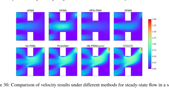 Figure 30. Comparison of velocity results under different methods for steady-state flow in a square cavity with obstructed segmented inlet at Reynolds number Re = 500
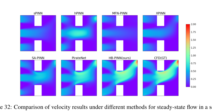 Figure 32. Comparison of velocity results under different methods for steady-state flow in a square cavity with obstructed segmented inlet at Reynolds number Re = 1000