Layered KIK quantum error mitigation for dynamic circuits

Background & Academic Lineage

The Origin & Academic Lineage

The problem addressed in this paper originates from the ongoing challenge of building reliable quantum computers in the Noisy Intermediate-Scale Quantum (NISQ) era and beyond. While Quantum Error Correction (QEC) is the ultimate goal for fault-tolerant quantum computing, it demands substantial hardware overhead, specifically a significant increase in the number of qubits. This makes QEC impractical for current and near-term devices.

As a more immediate and practical solution, Quantum Error Mitigation (QEM) emerged. QEM aims to reduce the impact of noise on quantum computation results without requiring the extensive hardware of QEC. Instead, QEM typically incurs a runtime cost, manifesting as an increased number of "shots" (repetitions) needed to achieve a desired accuracy. However, QEM itself faces scalability issues; its sampling overhead grows exponentially with circuit volume, limiting its applicability to circuits with up to about a hundred qubits.

A critical "pain point" of many early QEM approaches was their sensitivity to noise drifts. Noise parameters in quantum systems, such as decoherence times or coherent error magnitudes, often vary over the course of an experiment. Since QEM methods can significantly increase experiment runtimes, these temporal noise drifts can substantially degrade the final results. Characterization-based QEM methods, which rely on precisely learning the noise profile, are particularly vulnerable because the time required for accurate characterization often conflicts with the speed at which noise parameters drift.

This led to the development of agnostic (characterization-free) QEM methods, such as Zero-Noise Extrapolation (ZNE) and the Adaptive KIK protocol, which are inherently more resilient to noise drifts. The Adaptive KIK method, introduced in prior work [61], showed significant promise due to its drift resilience, applicability to non-Clifford gates, and guaranteed performance bounds. It was identified as a strong candidate for integration with QEC, forming hybrid QEC-QEM approaches that could leverage QEC for dominant, local errors and QEM for residual, correlated, or coherent errors that QEC struggles with.

However, the original Adaptive KIK protocol (referred to as Global KIK or GKIK) had two fundamental limitations that prevented its seamless integration with QEC and dynamic circuits:
1. Incompatibility with mid-circuit measurements (MCMs): MCMs are essential for executing syndrome measurements in QEC protocols, allowing errors to be detected and corrected during the computation. The global noise amplification strategy of GKIK was not compatible with these intermediate measurements.
2. Residual bias from high-order Magnus noise terms: The GKIK formulation neglected higher-order terms in the Magnus expansion, which could introduce a small but significant bias, especially when dealing with strong noise or when very high accuracy was required. This bias could lead to inaccurate mitigation results.

These limitations forced the authors to develop the Layered KIK (LKIK) method, which is specifically designed to overcome these hurdles by adopting a layer-based noise amplification approach, making it compatible with dynamic circuits and mid-circuit measurements, and addressing the high-order Magnus noise terms more effectively.

Intuitive Domain Terms

1. Quantum Error Mitigation (QEM):

   • Intuitive analogy: Imagine you're trying to take a very precise photo with a slightly blurry camera. QEM is like taking several photos, maybe even intentionally making some of them a bit blurrier in controlled ways, and then using a special computer program to combine them and guess what the perfectly clear photo should have looked like. You're not fixing the camera lens, but you're getting a better picture despite its flaws.

2. Quantum Error Correction (QEC):

   • Intuitive analogy: Think of sending a secret message by writing it on three separate pieces of paper and giving them to three different messengers. If one messenger loses their paper or it gets smudged, you can still reconstruct the original message from the other two. QEC is like having a system that not only tells you if a messenger's paper is damaged but also helps you fix it or replace it, ensuring the message always arrives perfectly, but it requires more resources (more paper, more messengers).

3. Dynamic Circuits:

   • Intuitive analogy: Consider a recipe where the next step depends on the outcome of a previous taste test. If the soup is too salty (a "mid-circuit measurement" outcome), you add more water (a specific "gate" operation). If it's just right, you move to the next ingredient. A dynamic circuit is a quantum program that can change its path or operations based on measurements made during the computation, rather than following a fixed, predetermined sequence.

4. Noise Drift Resilience:

   • Intuitive analogy: If you're trying to paint a straight line on a moving boat, "noise drift resilience" means your painting technique can adapt to the boat's constant, unpredictable swaying and still produce a straight line. It doesn't require you to stop the boat or constantly re-measure its movement; it just keeps the line straight despite the changing conditions.

5. Magnus Expansion:

   • Intuitive analogy: Imagine trying to predict the exact trajectory of a billiard ball, considering not just the initial hit but also tiny imperfections on the table, slight air resistance, and the ball's spin. The Magnus expansion is a mathematical tool that helps describe the ball's path by adding increasingly subtle corrections for these imperfections. "High-order Magnus noise terms" are like those very tiny, almost imperceptible effects that, while small, can become important if you need an extremely accurate prediction of where the ball will end up.

Notation Table

Notation	Description

Problem Definition & Constraints

Core Problem Formulation & The Dilemma

The current landscape of quantum computing experiments is plagued by noise, which introduces bias into the expectation values obtained from quantum circuits. While Quantum Error Mitigation (QEM) offers a practical pathway to address this, existing methods, particularly the Global KIK (GKIK) protocol, face significant limitations that hinder their applicability and scalability.

The Input/Current State is characterized by noisy quantum circuits, where the GKIK protocol, despite its advantages like drift resilience, suffers from several critical flaws:
* Incompatibility with Mid-Circuit Measurements (MCMs): GKIK's reliance on "global noise amplification" (Page 2) makes it fundamentally incompatible with MCMs (Page 5). MCMs are essential for dynamic quantum circuits and are a cornerstone of Quantum Error Correction (QEC) protocols, as they involve projective measurements that completely decohere the state. Treating these as "infinitely strong noise" within the global folding framework leads to incorrect noise amplification, as the projection effect is an intended part of the ideal dynamic circuit and should not be mitigated (Page 10).
* Bias from High-Order Magnus Noise Terms: The GKIK formulation neglects "high-order Magnus noise terms" (Page 2), resulting in a "small bias" in the mitigated expectation values (Page 5). This bias becomes substantial when dealing with strong noise or when "high accuracy is required" (Page 10).
* Hamiltonian Inversion Difficulty: GKIK requires "inverting the sign of the effective Hamiltonian," which is "not trivial to implement" on certain quantum computing platforms (Page 9).

Furthermore, characterization-based QEM methods, when considered for integration with QEC, encounter their own set of problems. Logical qubits, the output of QEC, exhibit "minuscule" error rates (Page 5). Characterizing these tiny errors for mitigation becomes "time-consuming" and demands "high-accuracy noise characterizations" (Page 4-5), making such integration impractical.

The Desired Endpoint (Output/Goal State) is a QEM method that is "drift-resilient and bias-free" for gate error mitigation in "dynamic circuits" (Page 9). Specifically, this method must:
* Be "compatible with mid-circuit measurements" (Page 2, Page 5).
* Effectively suppress "residual errors due to unaccounted high-order Magnus noise terms" (Page 2), ensuring high accuracy even in strong noise scenarios.
* Enable "seamless integration with quantum error correction codes" (Page 2), allowing QEC to handle dominant noise while the QEM addresses residual and correlated errors.
* Achieve these improvements "without incurring additional overhead or experimental complexity" compared to the original GKIK protocol (Page 2, Page 9).
* Be able to reduce the residual mitigation error below a "target experimental accuracy" by adjusting the number of layers (Page 17).

The Exact Missing Link or Mathematical Gap between the current state and the desired endpoint lies in developing a QEM protocol that can systematically address the $\Omega_2$ bias and integrate MCMs without compromising the mitigation process or incurring excessive overhead. The paper proposes a "layer-based application of KIK" (LKIK) to bridge this gap. Mathematically, the performance of GKIK is limited by the second-order Magnus term $\Omega_2^G$ of the entire circuit (Page 17). The LKIK approach aims to eliminate the cross-layer commutator contributions to $\Omega_2$ and make the remaining $\Omega_2$ contributions negligible by increasing the number of layers, thereby achieving a bias-free operation (Page 17). The challenge is to formulate this layered approach such that it correctly amplifies noise for each layer while preserving the functionality of MCMs and canceling higher-order noise terms.

The Painful Trade-off or Dilemma that has trapped previous researchers trying to solve this specific problem manifests in several ways:
1. QEM Runtime vs. Noise Drift: Many QEM protocols significantly increase the experiment's runtime, which, in turn, amplifies the impact of "temporal noise drifts" (Page 4). Methods relying on noise characterization are particularly vulnerable, as their characterization becomes outdated during long experimental runs (Page 4).
2. QEC Integration with Characterization-Based QEM: The desire to combine QEC with QEM is strong, but characterization-based QEM requires errors to be sufficiently pronounced and simple in structure for efficient learning. This clashes with the "minuscule" and complex errors expected on logical qubits after QEC, leading to "time-consuming high-accuracy noise characterizations" (Page 4-5). This creates a dilemma where improving QEC makes QEM integration harder.
3. GKIK's Global Amplification vs. Mid-Circuit Measurements: The global nature of GKIK's noise amplification is fundamentally at odds with the localized, state-projecting nature of MCMs. MCMs are an integral part of dynamic circuits and QEC, but GKIK's framework cannot correctly handle them, leading to "incorrect noise amplification" if MCMs are treated as part of the circuit to be inverted (Page 10). This is a core dilemma for achieving QEC-QEM integration with GKIK.
4. Accuracy/Noise Strength vs. Sampling Cost: Achieving high accuracy or mitigating strong noise with GKIK requires accounting for "high-order Magnus noise terms." However, the sampling cost required to address these terms can become "unrealistic" (Page 10), creating a trade-off between desired performance and experimental feasibility.

Constraints & Failure Modes

The problem of robust quantum error mitigation for dynamic circuits is made "insanely difficult" by several harsh, realistic walls:

• Physical Constraints:

  • Hamiltonian Inversion Complexity: The GKIK method requires "inverting the sign of the effective Hamiltonian" (Page 9). This is not a universally trivial operation and can be challenging to implement on various quantum computing platforms, especially for complex gates or architectures.
  • Control Electronics Speed for Thin Layers: While LKIK offers advantages, using "thinner layers" (i.e., dividing the circuit into many small segments) may necessitate "faster control electronics" due to more frequent sign changes of the drive Hamiltonian (Page 25). This imposes a hardware limitation on the granularity of layers.
  • Leakage Noise and Excitations in Thin Layers: For "thinner layers," there is an increased "potential for leakage noise and excitations of non-computational states" (Page 25). Mitigating these requires additional pulse shaping techniques, adding complexity to the experimental setup.

• Computational/Sampling Constraints:

  • Exponential Sampling Overhead of QEM: Most QEM methods, including KIK, incur a "sampling overhead" that grows "exponentially" with the circuit volume (Page 3). This limits their applicability to circuits with a relatively small number of qubits (e.g., up to a hundred in superconducting circuits).
  • Time-Consuming Noise Characterization: Characterization-based QEM methods require precise knowledge of noise parameters. For "minuscule" errors, such as those on logical qubits, this leads to "time-consuming high-accuracy noise characterizations" (Page 4-5), making them impractical for real-time applications or large circuits.
  • Unrealistic Sampling Costs for High Accuracy: When noise is strong or "very high accuracy is needed," the sampling cost required to account for high-order Magnus noise terms can become "unrealistic" (Page 10).
  • Exponential Overhead for Naive Layer-by-Layer Mitigation: A straightforward approach of mitigating each layer independently (e.g., by multiplying mitigated evolution operators for each layer) results in a sampling overhead that "grows exponentially with the number of layers" (Page 22). For instance, first-order mitigation of ten layers could require approximately one million ($2^{20}$) shots, which is often prohibitive.

• Data-Driven Constraints:

  • Temporal Noise Drifts: Noise parameters in quantum processors are not static; they "typically vary over time" due to factors like temperature fluctuations, stray electromagnetic fields, or two-level system defects (Page 4, Page 6). Since QEM experiments can run for "dozens of hours or more," these drifts can significantly impact the accuracy of mitigation (Page 6).
  • Requirements for Characterization-Based QEM: For characterization-based methods to be effective, errors must be "sufficiently pronounced to be learned within a reasonable timeframe with adequate accuracy," and the "noise structure be simple enough to be described using a small number of parameters" (Page 4-5). These conditions are often not met, especially for logical qubits.
  • Noisy Mid-Circuit Measurements: In practical quantum systems, MCMs are "often noisy," which can "lead to execution of the wrong gates" (Page 15). This introduces another layer of error that needs to be addressed, complicating dynamic circuits.

Failure Modes (if these constraints are not overcome or previous methods are used):
* Degraded Performance: If QEM protocols are not resilient to noise drifts, the final outcomes will be substantially impacted, leading to unreliable results (Page 4).
* Incorrect Results: Using methods like gate insertion for noise amplification, when the noise does not commute with the ideal unitary, leads to "incorrect amplifications" and biased results (Page 8, Page 20).
* Inability to Integrate QEC: The incompatibility of GKIK with MCMs means that QEC, which relies heavily on MCMs for syndrome measurements, cannot be seamlessly integrated, thus limiting the overall error suppression capabilities (Page 5, Page 10).
* Unachievable Accuracy: Neglecting high-order Magnus terms in GKIK means that achieving very high accuracy or mitigating strong noise becomes impossible without incurring "unrealistic" sampling costs (Page 10).
* Scalability Bottleneck: The exponential sampling overhead of many QEM methods, if not addressed, prevents their application to larger, more complex quantum circuits, limiting the scalability of quantum computation (Page 3).

Why This Approach

The Inevitability of the Choice

The Layered KIK (LKIK) approach emerges as the only viable solution by directly addressing critical limitations of prior quantum error mitigation (QEM) methods, including the previously most promising Global KIK (GKIK) protocol. Traditional "state-of-the-art" (SOTA) methods, such as characterization-based QEM (e.g., probabilistic error cancellation, Clifford regression, machine learning), were deemed insufficient because they are inherentely sensitive to temporal noise drifts. Noise parameters in quantum systems typically vary over time, and the substantial sampling overhead incurred by QEM methods means experiments can run for dozens of hours, making these drifts a significant obstacle (Page 4, Page 6). Furthermore, characterization-based methods struggle with the minuscule error rates expected in logical qubits, leading to impractically long characterization times and incompatibility with quantum error correction (QEC) requirements (Page 5).

Agnostic noise amplification methods, while more drift-resilient, also presented significant drawbacks. Pulse-stretching zero-noise extrapolation (ZNE) requires intricate calibration and is incompatible with twirling techniques that mis-scale coherent errors. Digital ZNE suffers from a strong error bias when noise does not commute with the ideal unitary operation, which is often the case. NOX, being a first-order mitigation theory, is limited to weak noise scenarios (Page 4).

The Adaptive KIK method (GKIK) was identified as a strong candidate for drift-resilient QEM and QEC integration, offering convergence assurances for non-strong noise. However, GKIK itself had two critical intrinsic hurdles that prevented its universal applicability:
1. Incompatibility with mid-circuit measurements (MCMs): MCMs are essential for executing syndrome measurements in QEC protocols. GKIK's global folding approach treats MCMs as "infinitely strong noise" that completely decohere the state, making them impossible to mitigate within its framework without altering the ideal dynamic circuit functionality (Page 5, Page 10).
2. Residual bias from high-order Magnus noise terms: GKIK exhibited a small, yet significant, bias due to unaccounted high-order Magnus expansion corrections. This bias becomes problematic when noise is strong or when high accuracy is required (Page 5, Page 9, Page 10).

The authors realized that to overcome these two specific hurdles simultaneously, while retaining the crucial drift-resilience and agnostic nature of KIK, a layer-based application was necessary. This realization led to the development of Layered KIK (LKIK), which is explicitly designed to resolve these issues and open a path towards truly drift-resilient and bias-free QEC-QEM protocols (Page 9).

Comparative Superiority

Layered KIK (LKIK) offers qualitative superiority over previous methods, including Global KIK (GKIK), primarily through its enhanced bias suppression and inherent compatability with dynamic circuits.

Firstly, LKIK significantly improves bias suppression. GKIK, while effective, suffered from a residual bias due to high-order Magnus noise terms (Page 5, Page 10). LKIK, by dividing the circuit into layers and applying KIK amplification layer-by-layer, systematically suppresses these high-order corrections. The analysis shows that the contribution from cross-layer commutators (represented by square regions in Figure 2) is eliminated, and the layer-specific second-order Magnus terms (blue triangles in Figure 2) become negligible as the number of layers ($L$) increases (Page 17, Page 18). This leads to a "bias-free" method in practice, meaning that for any target accuracy, a sufficiently large $L$ can be chosen to reduce the residual bias below the target experimental accuracy (Page 18). Quantitatively, for thin layers, the residual error scales as $1/L^2$ (Page 19, Figure 3), which is "substantially faster" than the $1/L$ coarse bound, demonstrating a superior structural advantage in error reduction.

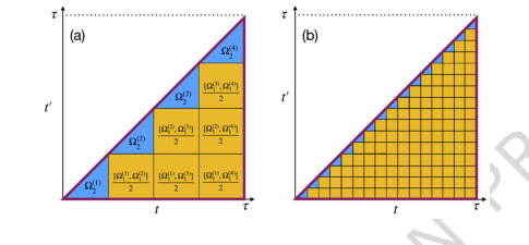Figure 2. Local contributions to the global Ω2. (a) & (b) The performance of the global KIK introduced in [61] is limited by the second-order Magnus term of the entire circuit, ΩG 2 . ΩG 2 is calculated using a double integral whose inte- gration domain is depicted by the big triangle in (a). τ is the time duration of the unmitigated circuit. The same circuit can be described as a sequence of L consecutive layers (L = 4 in (a)). As a result, ΩG 2 can be divided into two different types of contributions: i) the blue triangles that arise from the Ω2 of each layer, and ii) the orange squares which originate from the Ω1 commutator of different layers. Crucially, we show that in the layered KIK protocol, the contribution of the squares is eliminated, leaving only the blue triangles con- tribution. Furthermore, as the layers get thinner (b), the contribution of the blue triangles becomes negligible. From this argument one can derive an upper bound on the LKIK mitigation error that scales as 1/L. Interestingly, when the layers are sufficiently thin, we find a tighter error bound that scales as 1/L2. As such, LKIK is bias-free in practice, since it is always possible to choose a sufficiently large L that guarantees that the residual mitigation error remains below the target experimental accuracy

Secondly, LKIK's design inherently supports mid-circuit measurements (MCMs) and dynamic circuits, a critical structural advantage over GKIK. GKIK's global folding approach was incompatible with MCMs because they represent projective operations that cannot be globally inverted or amplified without corrupting the ideal circuit (Page 10). LKIK overcomes this by treating MCMs as unscaled functions within the layered mitigation framework. This allows MCMs to be incorporated without mitigation, preserving their ideal functionality within dynamic circuits (Page 15, Equations 22, 23, Figure 4). This is a crucial distinction, as dynamic circuits, including QEC codes, rely heavily on MCMs.

Finally, LKIK retains the key advantage of drift-resilience from the original KIK protocol. This means it can handle temporal variations in noise parameters, such as changes in decoherence times or coherent errors, without degradation in performance (Page 4, Page 8). This is a significant qualitative advantage over characterization-based QEM methods, which are inherently sensitive to such drifts (Page 4, Page 6). The combination of drift-resilience, bias-free operation, and MCM compatibility makes LKIK overwhelmingly superior for integrating QEM with QEC and for general dynamic circuits in the noisy intermediate-scale quantum (NISQ) era.

Alignment with Constraints

The Layered KIK (LKIK) method perfectly aligns with the harsh requirements of quantum error mitigation for dynamic circuits, effectively marrying the problem's constraints with the solution's unique properties.

1. Compatibility with Dynamic Circuits and Mid-Circuit Measurements (MCMs): A primary constraint was to develop a QEM method applicable to any dynamic circuit, including those with MCMs, which are fundamental to QEC. GKIK failed here due to its global folding approach (Page 5, Page 10). LKIK's layer-based amplification scheme directly resolves this. By applying KIK amplification to individual layers, MCMs can be incorporated as unscaled operations that are not mitigated, thus preserving their ideal functionality within the dynamic circuit (Page 15, Equations 22, 23). This is a perfect fit, as demonstrated by numerical simulations showing LKIK performs equally well for unitary evolution and dynamic circuits with MCMs and feedforward (Figure 4, Page 21).

2. Drift Resilience: A key desired feature for QEM protocols is resilience to noise drifts, where noise parameters vary over the course of an experiment (Page 4). LKIK inherits this crucial property from the KIK protocol. The execution order of the amplification circuits is specifically structured to eliminate temporal noise drift effects, ensuring that the method's performance does not degrade even when noise parameters fluctuate (Page 8, Page 9). This directly addresses the constraint of operating reliably in real-world, drifting quantum hardware.

3. Mitigation of High-Order Noise Terms and Bias-Free Operation: A significant constraint for high-accuracy QEM is the presence of residual errors from high-order noise terms, which plagued GKIK (Page 5, Page 10). LKIK's layered approach systematically suppresses these terms. By eliminating contributions from cross-layer commutators and making layer-specific second-order Magnus terms negligible with a sufficient number of layers, LKIK achieves a "bias-free" mitigation in practice (Page 17, Page 18). The residual error scales as $1/L^2$ for thin layers, ensuring that the mitigation error can be driven below any target experimental accuracy by choosing an appropriate number of layers (Page 19). This directly addresses the need for high-accuracy mitigation even in the presence of strong noise.

4. Seamless Integration with Quantum Error Correction (QEC): The overarching goal was to enable reliable and drift-resilient error mitigation for circuits undergoing imperfect QEC (Page 3). Since QEC codes are instances of dynamic circuits, LKIK's compatibility with dynamic circuits and MCMs makes it seamlessly integrable with QEC. This allows QEC to handle dominant local, uncorrelated errors, while LKIK suppresses residual errors like leakage, correlated, and coherent errors that are challenging for QEC (Page 3, Page 15). This synergy provides a robust hybrid approach that aligns perfectly with the vision of enhancing the reliability of quantum computing experiments.

Rejection of Alternatives

The paper provides clear reasoning for rejecting other popular QEM approaches, highlighting their fundamental limitations in the context of dynamic circuits, drift resilience, and high-accuracy requirements.

• Characterization-Based QEM Methods (e.g., PEC, PEA, Clifford regression, Machine Learning): These methods were explicitly rejected due to their "inherent sensitivity to temporal noise drifts" (Page 4, Page 6). Noise parameters in quantum systems are not static; they can vary significantly over the long runtimes of QEM experiments, making characterization-based approaches unreliable as the learned noise model quickly becomes outdated. Furthermore, applying these methods to logical qubits, where errors are expected to be minuscule, would require "time-consuming high-accuracy noise characterizations" that are impractical (Page 5). They also pose challenges for QEC integration due to these characterization requirements.

• Zero-Noise Extrapolation (ZNE) Methods (e.g., Pulse-Stretching ZNE, Digital ZNE, NOX):

  • Pulse-stretching ZNE was deemed problematic because it "requires careful control and calibration procedures" and "is also not fully compatible with twirling techniques... since the stretching mis-scales coherent errors" (Page 4). This limits its practical applicability and effectiveness for certain noise types.
  • Digital ZNE suffers from a "strong error bias at any mitigation order when the noise does not commute with the ideal unitary – which is typically the case" (Page 4). The paper explicitly states that "digital noise amplification is correct only in the uncommon cases where the noise happens to commute with the ideal gate" (Page 7), making it generally unsuitable.
  • NOX was rejected for high-accuracy or strong noise scenarios because it "is a first order mitigation theory, and therefore it is limited to weak noise scenarios" (Page 4).

• Purification Methods: These approaches were considered but dismissed because they "involves hardware overhead and is restricted to limited noise models" (Page 6). The goal was a method without additional hardware overhead and broader applicability.

• Global KIK (GKIK): While GKIK was a strong candidate for drift-resilient QEM, it was ultimately rejected as the final solution due to two critical flaws (Page 5, Page 9, Page 10):

  1. Incompatibility with mid-circuit measurements (MCMs): GKIK's global folding mechanism cannot properly handle MCMs, which are essential for dynamic circuits and QEC syndrome measurements. MCMs act as "infinitely strong noise" that cannot be described within the global folding framework without corrupting the ideal circuit (Page 10).
  2. Residual bias from high-order Magnus noise terms: GKIK exhibited a small, persistent bias that became significant for strong noise or when very high accuracy was required (Page 10). This limitation meant it could not achieve truly bias-free mitigation.

The Layered KIK approach was developed specifically to overcome these identified shortcomings of all existing alternatives, providing a drift-resilient, bias-free, and dynamic circuit-compatible QEM solution without additional hardware overhead.

Mathematical & Logical Mechanism

The Master Equation

The core mathematical engine of the Layered KIK (LKIK) quantum error mitigation method, as presented in this paper, revolves around constructing a mitigated evolution operator by combining amplified noisy circuits in a linear fashion. The central equation for the LKIK mitigated evolution operator, generalized for $L$ layers and up to mitigation order $M$, is given by:

$$ K_{\text{mit,LKIK}}^{(M)} = \sum_{j=0}^M a_j^{(M)} \prod_{l=1}^L K_l(K_l^I K_l)^j $$

Once this mitigated operator is constructed, the final mitigated expectation value for an observable $A$ on an initial state $\rho_0$ is obtained by:

$$ A_{\text{mit}}^{(M)} = \sum_{j=0}^M a_j^{(M)} \langle A | \left( \prod_{l=1}^L K_l(K_l^I K_l)^j \right) | \rho_0 \rangle $$

Term-by-Term Autopsy

Let's dissect these equations to understand each component:

• $K_{\text{mit,LKIK}}^{(M)}$: This is the Layered KIK mitigated evolution operator of order $M$.

  • Mathematical Definition: It's a linear combination of products of amplified noisy layer operators.
  • Physical/Logical Role: This operator represents the best estimate of the ideal, noise-free evolution operator $U$ after applying the LKIK mitigation protocol. Its goal is to effectively "undo" the noise present in the quantum circuit.
  • Why summation: The summation is used to form a polynomial approximation of the inverse noise channel. Each term in the sum contributes to a higher-order correction, allowing for a more accurate mitigation as $M$ increases.

• $M$: This denotes the mitigation order.

  • Mathematical Definition: An integer representing the highest power of noise amplification included in the linear combination.
  • Physical/Logical Role: A higher $M$ implies a more sophisticated polynomial approximation of the inverse noise, leading to potentially better error mitigation but also increased sampling overhead.

• $a_j^{(M)}$: These are the coefficients for the linear combination.

  • Mathematical Definition: Real numbers, typically derived from a Taylor expansion (Taylor coefficients, as in Eq. (4)) or adaptively determined by minimizing an L2 norm (adaptive coefficients, mentioned in Ref. [61]).
  • Physical/Logical Role: These coefficients are crucial for ensuring that the linear combination of amplified noisy circuits effectively approximates the ideal, noise-free evolution. They are designed to cancel out noise terms up to a certain order. The paper primarily focuses on Taylor coefficients, which are analytically derived and not learned.
  • Why addition: The coefficients are added because they form a linear combination, which is the mathematical structure for polynomial approximation.

• $\prod_{l=1}^L$: This represents a product over layers.

  • Mathematical Definition: A sequential composition of operators, ordered from $l=1$ to $L$.
  • Physical/Logical Role: This signifies that the quantum circuit is divided into $L$ distinct, non-overlapping layers. The overall circuit evolution is the sequential application of these layer evolutions. The product ensures that the time-ordering of operations is respected, which is vital in quantum mechanics.

• $K_l$: This is the noisy evolution operator for layer $l$.

  • Mathematical Definition: An operator (in Liouville space) that describes the actual, imperfect quantum evolution of the $l$-th layer, including both the ideal unitary operation and the noise.
  • Physical/Logical Role: This is the fundamental building block of the noisy circuit. It's what we're trying to mitigate errors from.

• $K_l^I$: This is the pulse-inverse of $K_l$.

  • Mathematical Definition: An operator obtained by reversing the schedule of the effective interaction Hamiltonian for layer $l$ and inverting its sign.
  • Physical/Logical Role: The pulse-inverse is a critical component of the KIK protocol. It's designed to "undo" the ideal unitary part of $K_l$ while preserving or amplifying the noise in a controlled manner. This allows for the construction of noise-amplified circuits.

• $(K_l^I K_l)^j$: This term represents the amplified noise for layer $l$ at amplification factor $j$.

  • Mathematical Definition: The operator $K_l^I K_l$ applied $j$ times.
  • Physical/Logical Role: The product $K_l^I K_l$ is designed such that its ideal part is the identity, but its noisy part is amplified. Repeating this $j$ times further amplifies the noise. This controlled amplification is the core idea behind noise amplification-based error mitigation.

• $\langle A | \cdot | \rho_0 \rangle$: This denotes the expectation value of an operator.

  • Mathematical Definition: In Liouville space, for an operator $O$, the expectation value is $\text{Tr}[A \cdot O(\rho_0)]$, where $A$ is the observable and $\rho_0$ is the initial state. The notation $\langle A | O | \rho_0 \rangle$ is a compact way to express this.
  • Physical/Logical Role: This is the final quantity of interest in a quantum experiment – the average value of a measurement. The goal of mitigation is to make this value as close as possible to the ideal, noise-free expectation value.

Step-by-Step Flow

Imagine a quantum computation as a complex machine, and LKIK as a sophisticated repair and calibration process. Here's how a single abstract data point (representing the quantum state) flows through this mechanism:

1. Circuit Disassembly: First, the original, full quantum circuit, which performs a desired computation but is inherently noisy, is conceptually broken down into $L$ smaller, sequential "layers" ($K_1, K_2, \dots, K_L$). Each layer $K_l$ is itself a noisy operation.

2. Layer-Specific Noise Amplification: For each individual layer $K_l$, the protocol generates a series of "amplified" versions. This involves creating a special "pulse-inverse" circuit, $K_l^I$, which is designed to effectively reverse the ideal part of $K_l$. Then, for each layer $l$ and for various amplification factors $j$ (from $0$ to $M$), a noise-amplifying block $(K_l^I K_l)^j$ is constructed. When $j=0$, this block is just the identity. When $j=1$, it's $K_l^I K_l$, and so on. The key here is that $K_l^I K_l$ amplifies the noise without changing the ideal unitary functionality.

3. Reassembly into Amplified Full Circuits: Next, for each mitigation order $j$, a complete, full-length quantum circuit is reassembled. This reassembled circuit is formed by concatenating the original noisy layer $K_l$ with its noise-amplamplifying block $(K_l^I K_l)^j$, for each layer $l$. The full circuit for a given $j$ looks like $K_L(K_L^I K_L)^j \dots K_2(K_2^I K_2)^j K_1(K_1^I K_1)^j$. This process generates $M+1$ distinct full circuits, each with a different level of noise amplification across all its layers.

4. Execution and Measurement: Each of these $M+1$ specially constructed circuits is then executed on the quantum computer, starting with the initial state $\rho_0$. For each execution, the expectation value of the observable $A$ is measured. This yields a set of raw, noisy expectation values, $A_0^{\text{raw}}, A_1^{\text{raw}}, \dots, A_M^{\text{raw}}$.

5. Post-processing (Linear Combination): Finally, these raw expectation values are fed into a classical computer. Here, they are combined using a pre-determined set of coefficients, $a_j^{(M)}$. The final mitigated expectation value, $A_{\text{mit}}^{(M)}$, is calculated as a weighted sum: $A_{\text{mit}}^{(M)} = \sum_{j=0}^M a_j^{(M)} A_j^{\text{raw}}$. This linear combination acts as a filter, cancelling out the amplified noise terms to provide a better estimate of the true, noise-free expectation value.

Optimization Dynamics

The "optimization" in Layered KIK (LKIK) isn't a continuous, iterative learning process in the typical machine learning sense, but rather a strategic construction and post-processing scheme designed for convergence and bias reduction.

1. Polynomial Approximation for Noise Inversion: The fundamental idea is to approximate the inverse of the noise channel, $N^{-1}$, using a polynomial expansion. The coefficients $a_j^{(M)}$ are chosen such that the linear combination $\sum_{j=0}^M a_j^{(M)} N^{2j}$ effectively approximates $N^{-1}$. For the scope of this paper, these coefficients are primarily the Taylor coefficients, which are analytically derived (Eq. 4) from a Taylor expansion of $x^{-1}$ around $x=1$. Therefore, there is no "learning" or iterative update of these coefficients within this specific work. The coefficients are fixed once the mitigation order $M$ is chosen.

2. Convergence through Mitigation Order ($M$): The accuracy of the mitigation improves as the mitigation order $M$ increases. A higher $M$ means a higher-degree polynomial approximation for the inverse noise channel, which can cancel out more complex or higher-order noise terms. This leads to a more accurate mitigated expectation value, converging towards the ideal value. However, increasing $M$ also incurs a higher sampling overhead, as more circuits need to be executed.

3. Bias Reduction through Layering ($L$): A key innovation of LKIK is its ability to significantly reduce residual bias by dividing the circuit into $L$ layers. The paper demonstrates that the leading-order bias term, related to the second-order Magnus term $\Omega_2$, scales as $1/L^2$ for sufficiently thin layers (Eq. 34). This means that by increasing the number of layers $L$, the inherent bias of the mitigation method itself can be made arbitrarily small, making the protocol "bias-free" in practice for a sufficiently large $L$. This is a crucial convergence mechanism that is distinct from increasing $M$.

4. Drift Resilience Mechanism: The protocol is designed to be resilient to temporal noise drifts. This is achieved by structuring the experiment such that the total number of measurement shots is divided into multiple sets. Within each set, all the $M+1$ amplified circuits (for a given $M$) are executed. This ensures that any noise drift occurring during the experiment affects all circuits within a set in a similar manner. The linear combination (summation) in the post-processing step then effectively cancels out this common drift-induced bias from each set. Averaging the mitigated results over many such sets further reduces the variance, leading to a robust, drift-resilient outcome. This is a clever way to handle time-varying noise without needing to characterize it.

In summary, the LKIK mechanism "learns" in the sense that its coefficients are pre-computed to approximate an inverse function, and it "converges" by increasing the order of this approximation ($M$) and by reducing intrinsic bias through circuit layering ($L$). The method's robustness is further bolstered by its inherent drift resilience, which is a structural property of its execution protocol rather than an iterative optimization.

Results, Limitations & Conclusion

Experimental Design & Baselines

The authors rigorously validated their Layered KIK (LKIK) approach primarily through numerical simulations, with references to companion experimental work for specific aspects. The core experimental architecture to prove their mathematical claims involved comparing LKIK against the Global KIK (GKIK) method, which serves as the primary baseline.

For the main comparison, a four-qubit simulation was employed, as depicted in Figure 1. The experiment was designed to measure the difference $\Delta(A)$ between the mitigated expectation value and the ideal value, plotted against the mitigation order $M$. Order $M=0$ represented no mitigation. Two noise strength parameters were tested: a weaker noise scenario with $\xi = 0.02$ (Figure 1a) and a stronger noise scenario with $\xi = 0.2$ (Figure 1b). The ideal expectation value was set to approximately $0.025$. The "victims" in this comparison were GKIK (represented as "1 Layer (GKIK)") and LKIK with varying numbers of layers (2, 4, 10, 20 layers). This setup allowed for a direct comparison of how increasing the number of layers in LKIK impacted mitigation performance under different noise conditions.

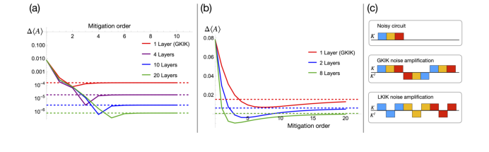Figure 1. A four-qubit simulation demonstrating the advantage of using the layered-based KIK (LKIK) amplification over the global KIK amplification (GKIK - single layer). In (a) & (b) the y axis is the difference ∆⟨A⟩be- tween the mitigated expectation value (see main text) and the ideal value, and the x axis is the mitigation order M with M = 0 indicating no mitigation. The ideal expectation value is ⟨A⟩≃0.025. In (a) the noise strength parameter is ξ = 0.02 and in (b) it is ξ = 0.2. Fig. (a) shows that LKIK is essential for achiev- ing high accuracy even when the noise is weak, while Fig. (b) shows that LKIK is important when the noise is strong even when the requested target accuracy is modest. The dashed lines show the prediction of the Layered KIK formula (30). (c) An illustration of a three-layer circuit (top) being noise amplified with GKIK (middle) and LKIK (bottom). The amplification factor is three for both cases. Squares below the black horizontal line represent pulse-inverse operation

To specifically demonstrate the scaling of the residual error, Figure 3 presented a numerical experiment for the same four-qubit circuit as in Figure 1a, but this time plotting the error for a fixed mitigation order (seven) as a function of the number of layers $L$. This was crucial for verifying the theoretical prediction of a $1/L^2$ error dependence for thin layers.

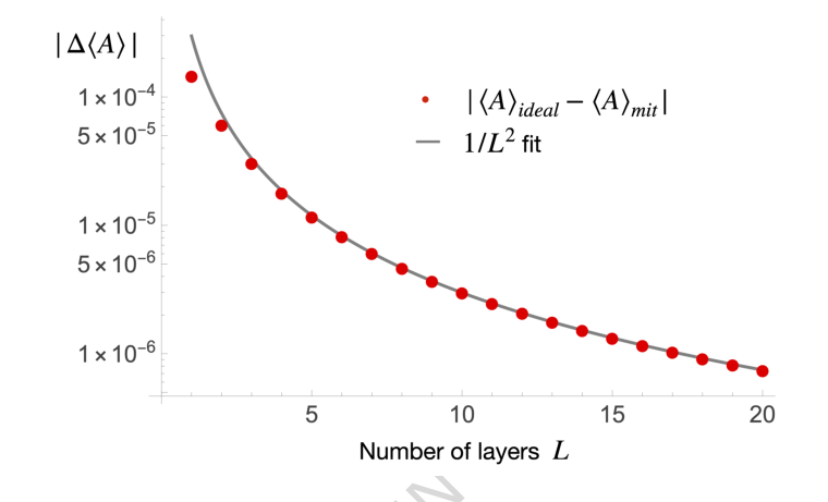Figure 3. For the same example as in Fig. 1a, the error with respect to the ideal expectation value (red dots) is plotted for order seven as a function of number of layers. The good fit to the 1/L2 curve confirms the prediction of Eq. (34)

Furthermore, the paper addressed LKIK's compatibility with dynamic circuits, which is a key advantage. Figure 4 showcased a numerical simulation comparing LKIK mitigation for a dynamic circuit (incorporating mid-circuit measurements and feedforward) against a non-dynamic, unitary evolution circuit. Both scenarios used 10 layers and a noise parameter of $\xi = 0.1$. This experiment aimed to definitively show that LKIK performs equally well in complex dynamic settings, where GKIK previously failed due to incompatibility with mid-circuit measurements.

While this paper primarily focuses on numerical evidence and analytical derivations for LKIK, it refers to two experimental demonstrations of the underlying KIK principles in its "Methods" section. Supplementary Note 1 describes an experiment on a trapped ion quantum computer (IBEX - AQT) that demonstrated the drift resilience of the KIK method by artificially inducing temporal over-rotations in an $R_{xx}(\pi/2)$ gate circuit. Supplementary Note 2 details an experiment on an IBM superconducting device (ibm_jakarta) that verified the issues of incorrect noise amplification arising from gate insertion, a problem that LKIK aims to resolve. The experimental validation of LKIK's effectiveness in mitigating errors in dynamic quantum circuits is explicitly stated to be presented in a companion paper [62].

What the Evidence Proves

The numerical evidence presented in this paper provides compelling proof for the advantages of Layered KIK (LKIK) over Global KIK (GKIK) and addresses several critical limitations of previous quantum error mitigation (QEM) schemes.

Firstly, the simulations in Figure 1 undeniably demonstrate that LKIK significantly outperforms GKIK in reducing the error $\Delta(A)$. For both weak ($\xi = 0.02$) and strong ($\xi = 0.2$) noise scenarios, increasing the number of layers in LKIK leads to a substantial decrease in the mitigated expectation value's deviation from the ideal. For instance, in Figure 1a, with $\xi = 0.02$, GKIK (1 layer) plateaus at an error around $10^{-3}$, while LKIK with 20 layers achieves an error below $10^{-5}$ at higher mitigation orders. This is definitive evidence that the layer-based noise amplification mechanism effectively suppresses errors that GKIK could not. The dashed lines in Figure 1, representing the prediction of the Layered KIK formula (Eq. 30), align well with the simulation results, further validating the underlying mathematical model.

Secondly, the paper provides strong evidence for the bias-free nature of LKIK with a sufficient number of layers. Figure 3, which plots the error for mitigation order seven against the number of layers, clearly shows that the error scales as $1/L^2$. The excellent fit of the red dots (simulation results) to the gray $1/L^2$ curve confirms the theoretical prediction (Eq. 34). This scaling is a crucial mathematical claim, proving that as the circuit is divided into more layers, the residual bias from high-order Magnus noise terms diminishes rapidly, making LKIK practically bias-free for a sufficiently large $L$. This directly addresses a major limitation of GKIK, which suffered from small residual errors due to unaccounted high-order Magnus terms.

Thirdly, LKIK's compatibility with dynamic circuits, including mid-circuit measurements (MCM) and feedforward, is a significant breakthrough. Figure 4 illustrates that LKIK performs equally well for a dynamic circuit (blue curve) and a non-dynamic, unitary evolution circuit (green curve). In both cases, the error $\Delta(A)$ approaches zero with increasing mitigation order. This is a hard piece of evidence that LKIK overcomes GKIK's incompatibility with MCMs, which are essential for quantum error correction (QEC) protocols. This makes LKIK a viable QEM method for complex, real-world quantum computations.

Finally, while not directly shown in new experimental results within this paper, the text emphasizes that LKIK inherits the drift-resilience of the original KIK protocol, as demonstrated in Supplementary Note 1. This means the method's performance is robust against temporal variations in noise parameters, a critical feature for long-running quantum experiments. The combination of bias-free operation, dynamic circuit compatibility, and drift resilience makes LKIK a powerful and versatile QEM approach.

Limitations & Future Directions

While the Layered KIK (LKIK) protocol presents a significant advancement in quantum error mitigation, it's important to acknowledge its current limitations and consider avenues for future development.

One immediate limitation is that this manuscript is an "ARTICLE IN PRESS," meaning it's an unedited version and may contain errors. From a technical standpoint, while LKIK is designed to be drift-resilient and bias-free, its reliance on pulse-based inverse protocols (KIK component) might not be universally straightforward to implement across all quantum computing platforms and gate types. Specifically, the paper notes that implementing the pulse inverse for fixed or tunable coupler phase gates [72] is "less straightforward." This suggests that hardware-level control and calibration remain a practical challenge for broad applicability.

Another aspect to consider is the sampling overhead. Although LKIK, especially with adaptive coefficients, can reduce the sampling cost compared to other methods, it still incurs a non-trivial overhead. The paper mentions "sampling overheads on the order of ten thousand or more are realistic for QEM protocols which are drift-resilient." While this is deemed realistic, it still represents a significant resource cost, particularly as circuit complexity grows. The comparison with multi-variate extrapolation (MVE) also highlights that MVE, despite a smaller depth overhead, incurs a "significantly larger sampling overhead" than single-layer Taylor (SLT) with GKIK, implying that optimizing runtime and sampling efficiency remains a crucial area.

Furthermore, the theoretical error scaling of $1/L^2$ for LKIK relies on the assumption of "sufficiently thin, uniformly-spaced layers." While the paper shows that deviations from uniformity only slightly affect the coarser $1/L$ bound, achieving the optimal $1/L^2$ scaling in practice might require careful circuit decomposition and pulse-level control. The experimental validation of LKIK for dynamic circuits, as mentioned, is primarily in a companion paper [62], meaning the direct experimental evidence for all claims within this paper is not fully detailed here.

Looking ahead, several exciting discussion topics and research directions emerge:

1. Deeper QEC-QEM Integration: The seamless compatibility of LKIK with mid-circuit measurements opens the door for truly robust hybrid QEC-QEM protocols. Future work could focus on designing and experimentally demonstrating integrated systems where QEC handles the dominant, local, uncorrelated errors, and LKIK then mitigates the residual, harder-to-correct errors like leakage, correlated noise, and coherent errors. This could significantly push the boundaries of fault-tolerant quantum computing.

2. Optimizing Layer Decomposition and Adaptive Coefficients: How can we optimally determine the number and structure of layers ($L$) for a given quantum circuit and noise profile? Research could explore adaptive algorithms for layer decomposition that dynamically adjust $L$ to minimize total overhead while meeting target accuracy. Further development of the adaptive post-processing techniques, which were deferred in this work, is essential to achieve stronger mitigation with fewer shots and circuits.

3. Hardware-Specific Implementations and Pulse Engineering: Investigating the specific challenges and solutions for implementing pulse-inverse operations for various gate sets on different quantum hardware architectures (e.g., superconducting, trapped-ion, photonic). This could involve advanced pulse shaping techniques to mitigate leakage noise and excitations in thinner layers, ensuring the method's practicality across diverse platforms.

4. Mitigation of Non-Markovian Effects: While Pauli twirling and pseudo-twirling can address non-Markovian noise before applying KIK, exploring methods to directly incorporate non-Markovian noise models into the LKIK framework itself could lead to even more powerful and general mitigation strategies. This would require a deeper understanding of how non-Markovian dynamics propagate through layered circuits.

5. Synergy with Other QEM Methods: The paper suggests combining LKIK with characterization-based methods (PEC, PEA, machine learning) to tackle the "bulk" of the noise, allowing LKIK to focus on drifts and errors outside sparse noise models. Future research could systematically explore these hybrid approaches, quantifying the trade-offs in sampling overhead, drift resilience, and overall performance. For instance, combining LKIK with Tensor Error Mitigation (TEM) could potentially yield a noise-drift resilient solution with a smaller sampling overhead than LKIK alone.

6. Runtime Overhead and Scalability: A detailed analysis and experimental validation of the runtime overhead for LKIK, especially in comparison to other advanced QEM methods like MVE, is crucial for assessing its practical scalability. Exploring parallelization strategies for shot collection across multiple quantum processors could further reduce wall-clock time, making high sampling overheads more manageable.

By addressing these limitations and exploring these future directions, the LKIK framework has the potential to become a cornerstone for reliable quantum computation in the noisy intermediate-scale quantum (NISQ) era and beyond.