RFWave: Multi-band Rectified Flow for Audio Waveform Reconstruction

Background & Academic Lineage

The Origin & Academic Lineage

The problem of audio waveform reconstruction, which involves transforming low-dimensional features into realistic, perceptible sounds, emerged from the growing demand for enhanced digital interractions. This technology is cruciall for diverse applications such as virtual assistants, entertainment systems, and text-to-speech synthesis, where generating high-quality, natural-sounding voice and music is paramount. Historically, this field moved beyond traditional signal processing methods (Kawahara et al., 1999; Morise et al., 2016) with the advent of advanced generative modells.

Early significant advancements came from two main paradigms: autoregressive models and Generative Adversarial Networks (GANs) (Goodfellow et al., 2014). Autoregressive models, while capable of producing high-quality audio, were severely limited by their slow generation speeds. This slowness stemmed from their sequential prediction of individual sample points (Oord et al., 2016; Kalchbrenner et al., 2018; Valin & Skoglund, 2019), making real-time applications impractical. GANs offered faster generation by predicting sample points in parallel (Kumar et al., 2019; Yamamoto et al., 2020; Kong et al., 2020a), but they introduced their own set of "pain points." These included the necessity for complex discriminator designs and issues like training instability or mode collapse (Thanh-Tung et al., 2018), where the model might fail to learn the full diversity of the data.

More recently, diffusion models (Song et al., 2020; Ho et al., 2020) emerged as a promising alternative, offering greater training stability and the ability to reconstruct high-quality waveforms (Chen et al., 2020; Kong et al., 2020b; gil Lee et al., 2022). However, diffusion models inherited a significant limitation: they were at least an order of magnitude slower than GANs. This slowness was primarily due to two factors: (1) the requirement of numerous sampling steps to achieve high-quality samples, and (2) their operation at the individual waveform sample point level. The latter often involved multiple upsampling operations to bridge frame rate and sample rate resolutions, leading to increased sequence length, higher GPU memory usage, and substantial computational demands. This fundamental limitation of slow inference speed in diffusion models is the core "pain point" that RFWave aims to address, striving to match GAN-based speeds while retaining diffusion models' stability and quality.

Intuitive Domain Terms

Here are some specialized terms from the paper, translated into everyday analogies for a beginner:

• Mel-spectrogram: Imagine you have a piece of sheet music that visually represents a song. A Mel-spectrogram is similar, but it's a digital "picture" of sound that a computer can understand. It shows how the loudness of different frequencies changes over time, with a special scaling (Mel scale) that mimics how humans perceive pitch. It's like a musical score for a machine, highlighting the important parts of the sound.
• Rectified Flow: Think of a journey from point A to point B. Normally, you might take a winding road with many turns. Rectified Flow is like finding the most direct, straight-line path between point A (noisy data) and point B (clean audio). This "straight highway" makes the journey much faster and more efficient, allowing the model to transform noise into sound in fewer steps.
• Diffusion Models: Picture a very blurry photograph that gradually becomes clearer and sharper with each step you take to "denoise" it. Diffusion models work similarly: they start with random noise (like a completely blurry image) and slowly, step-by-step, transform it into a coherent, high-quality audio waveform by reversing a diffusion process. It's like an artist slowly adding detail to a canvas until a masterpiece emerges.
• Mode Collapse (in GANs): Imagine a chef who is asked to cook a variety of dishes but only learns to make one specific dish perfectly, ignoring all other recipes. In generative models like GANs, mode collapse means the model fails to generate diverse outputs and instead produces only a limited set of similar, high-quality samples. It's like the chef always making the same perfect pasta, even when asked for steak or salad, because it's the only thing it knows how to do well.

Notation Table

Notation	Description
$Z_t$	The evolving state of the data at a given time $t$ during the transformation process.
$v(Z_t, t)$	The "velocity" field that dictates how the data $Z_t$ changes at time $t$, guiding it towards the target.
$\pi_0$	The initial probability distribution, typically representing random noise.
$\pi_1$	The target probability distribution, representing the desired real audio data.
$X_0$	An initial data sample, usually random noise, drawn from $\pi_0$.
$X_1$	A target data sample, representing the ground truth audio waveform or spectrogram, drawn from $\pi_1$.
$X_t$	An intermediate data sample at time $t$, representing the interpolation between $X_0$ and $X_1$.
$t$	The time variable, which progresses from $0$ (start of transformation) to $1$ (end of transformation).
$C$	Conditional input, such as a Mel-spectrogram or discrete acoustic tokens, that guides the audio generation.
$N$	The size of the Fast Fourier Transform (FFT), determining the frequency resolution.
$d_s$	The number of frequency bins within a specific subbands' complex spectrum.
$F$	The total number of frames in a spectrogram, representing time segments.
$i_{sb}$	The index identifying a specific subband.
$i_{bw}$	The bandwidth index for EnCodec tokens, used for different compression levels.
$\sigma$	A weighting coefficient used in the energy-balanced loss, often derived from the standard deviation of the ground truth velocity.
$S(v)$	A measure of the "straightness" of the learned velocity field's trajectories, indicating how direct the transformation path is.

Problem Definition & Constraints

Core Problem Formulation & The Dilemma

The core problem addressed by this paper is the challenge of efficiently reconstructing high-fidelity audio waveforms from various compressed representations, such as Mel-spectrograms or discrete acoustic tokens.

The Input/Current State for this problem involves:
* Low-dimensional audio features, specifically Mel-spectrograms or discrete acoustic tokens, which are compact representations of sound.
* Existing generative models, primarily diffusion models and Generative Adversarial Networks (GANs), each with their own limitations. Diffusion models, while capable of producing high-quality audio, operate at the individual waveform sample point level and require numerous sampling steps, leading to significant latency. GANs, while faster, often suffer from training instability and mode collapse, and require complex discriminator designs.

The Desired Endpoint/Goal State is to achieve:
* High-fidelity audio waveforms reconstructed from these low-dimensional inputs.
* A generative model that matches the inference speed of GAN-based methods (i.e., real-time or faster) while retaining the training stability and high sample quality characteristic of diffusion models.
* The ability to reconstruct waveforms with a drastically reduced number of sampling steps (e.g., just 10 steps, as achieved by RFWave).
* Superior computational efficiency, enabling audio generation at speeds significantly faster than real-time (e.g., up to 160 times faster on a GPU).
* Versatility in reconstructing audio from both Mel-spectrograms and discrete acoustic tokens.

The exact missing link or mathematical gap between the current state and the desired endpoint is the absence of a generative modeling framework that can simultaneously achieve the high perceptual quality and training stability of diffusion models and the high computational efficiency and low latency of GANs for audio waveform reconstruction. Previous diffusion models are mathematically formulated to gradually denoise a signal over many steps, making them inherently slow. GANs, while fast, lack the robust mathematical guarantees for stable training and consistent quality. This paper attempts to bridge this gap by leveraging Rectified Flow, which aims to learn a direct, straight transport trajectory between noise and data distributions, thereby reducing the required sampling steps. Specifically, Rectified Flow learns a velocity field $v(Z_t, t)$ that governs the evolution of a noisy sample $Z_t$ from an initial noise distribution $\pi_0$ to a target data distribution $\pi_1$, such that $\frac{dZ_t}{dt} = v(Z_t, t)$. The learning objective minimizes the deviation from a straight-line trajectory:
$$ \min E_{(X_0, X_1)\sim\gamma} \int_0^1 || \frac{d}{dt}X_t - v(X_t, t) ||^2 dt $$
where $X_t = (1-t)X_0 + tX_1$ represents a linear interpolation. This mathematical formulation is the key to accelerating the inference process by enabling fewer, more direct steps.

The painful trade-off or dilemma that has trapped previous researchers is the fundamental conflict between audio quality/training stability and inference speed/computational efficiency. Improving one aspect typically degrades the other:
* Diffusion models: Offer excellent audio quality and stable training, but are notoriously slow. Their operation at the "individual sample point level" and the need for "numerous sampling steps" (often hundreds or thousands) lead to high latency and computational demands.
* GANs: Provide fast generation speeds by predicting sample points in parallel, but are plagued by "complex discriminator designs and issues like instability or mode collapse," making them harder to train reliably and sometimes leading to lower quality or less diverse outputs.

This dilemma means researchers previously had to choose between a high-quality, stable but slow model, or a fast but potentially unstable and lower-quality model. The paper aims to break this trade-off.

Constraints & Failure Modes

The problem of high-fidelity, real-time audio waveform reconstruction is insanely difficult due to several harsh, realistic constraints and inherent failure modes:

• Computational Cost and GPU Memory Limits:

  • Sample Point-Level Operation: Previous diffusion models process audio at the individual sample point level. This requires "multiple upsampling operations to transition from frame rate resolution to sample rate resolution, increasing the sequence length and consequently leading to higher GPU memory usage and computational demands" (Page 2). For high-resolution audio (e.g., 44.1 kHz or 48 kHz), processing millions of samples per second is computationally prohibitive and memory-intensive. For instance, PriorGrad can only train on 6-second audio clips at 44.1 kHz within 30 GB of GPU memory, highlighting this severe memory constraint (Page 4).
  • Numerous Sampling Steps: Diffusion models typically require hundreds or thousands of sampling steps to generate high-quality audio, directly impacting inference speed and computational load. This makes them "at least an order of magnitude slower compared to GANs" (Page 1).

• Real-time Latency Requirements: Many practical applications (e.g., virtual assistants, real-time communication) demand extremely low latency. Existing diffusion models, even the fastest ones, are only "about 10 to 20 times faster than real-time" (Page 3), which is insufficient for true real-time interaction, especially when combined with large-scale acoustic models.

• Training Instability and Mode Collapse (for GANs): While GANs offer speed, their training is notoriously difficult. "Complex discriminator designs" and issues like "instability or mode collapse" (Page 1) mean they can fail to learn the full data distribution, leading to less diverse or lower-quality outputs.

• Error Accumulation in Multi-band Processing: When using multi-band strategies, "conditioning higher bands on lower ones can lead to an error accumulation, which means inaccuracies in the lower bands can adversely affect the higher bands during inference" (Page 4). This means errors in one part of the frequency spectrum can propagate and corrupt others.

• Low-Volume Noise in Silent Regions: A common failure mode for models trained with Mean Square Error (MSE) loss is the presence of "low-volume noise in expected silent regions" (Page 5). This occurs because small errors in silent parts contribute minimally to the overall MSE, causing the model to prioritize reducing larger errors in high-amplitude regions, leading to perceptible noise in quiet sections.

• Inconsistencies Between Subbands: When different frequency subbands are predicted independently, there's a risk of "inconsistencies among them" (Page 6), leading to audible artifacts at the subband boundaries in the reconstructed waveform.

• Artifacts in Background Noise: Without specific loss functions like STFT loss, models can generate "vertical patterns" or other "artifacts in the presence of background noise" (Figure A.8, Page 6), degrading the perceived quality.

• Non-linear Transport Trajectories: The effectiveness of Rectified Flow relies on learning "straight transport trajectories" (Page 2). If the learned velocity field deviates significantly from linearity, the Euler method will require more steps to accurately approximate the ODE, negating the efficiency benefits. This makes learning the velocity field a delicate task.

Why This Approach

The Inevitability of the Choice

The core problem RFWave addresses is the critical trade-off between audio reconstruction quality and generation speed in generative models. Traditional state-of-the-art (SOTA) methods, while advanced, each presented significant limitations that made them insufficient for achieving both high-fidelity and real-time performance simultaneously.

The authors realized that standard diffusion models, despite their prowess in generating high-quality audio and offering stable training, were fundamentally hindered by two factors: (1) their operation at the individual waveform sample point level, and (2) the necessity for numerous sampling steps to achieve desired quality. This led to severe latency issues and high GPU memory consumption, making them at least an order of magnitude slower than GANs and impractical for real-time applications. The paper explicitly states this realization: "While diffusion models are adept at this task, they are hindered by latency issues due to their operation at the individual sample point level and the need for numerous sampling steps." (Abstract). This insufficiency was further underscored by the observation that even the fastest diffusion methods were only 10 to 20 times faster than real-time, a far cry from the demands of real-world applications.

Generative Adversarial Networks (GANs), while capable of faster generation speeds by predicting sample points in parallel, suffered from inherent training instability and issues like mode collapse, often requiring complex discriminator designs. Autoregressive models, another class of generative models, were similarly rejected due to their sequential prediction of sample points, leading to unacceptably slow generation speeds.

Rectified Flow, combined with a multi-band, frame-level processing strategy, emerged as the only viable solution because it directly tackles these fundamental limitations. It offers a mechanism to achieve the high sample quality and training stability of diffusion models while simultaneously matching and even exceeding the generation speed of GANs, all within practical memory constraints. The ablation study further reinforces this, showing that "Rectified Flow is critical for our model to efficiently generate high-quality audio samples" (Page 9), as traditional diffusion noise schedules with more steps fell short.

Comparative Superiority

RFWave demonstrates overwhelming qualitative superiority over previous gold standards, extending far beyond simple performance metrics.

Firstly, in terms of speed, RFWave achieves an inference speed of up to 160 times faster than real-time on a GPU (Abstract). This is a dramatic improvement over diffusion models, which typically operate at 10-20 times real-time, and even surpasses many GAN-based methods. For instance, Table 7 shows RFWave's GPU xRT (times real-time) at 162.59, compared to BigVGAN's 72.68 and PriorGrad's 16.67. This structural advantage stems from Rectified Flow's ability to learn straight transport trajectories, enabling high-quality reconstruction with just 10 sampling steps, a significantly lower number than other diffusion models.

Secondly, regarding quality, RFWave consistently outperforms diffusion-based baselines like PriorGrad and FreGrad in both objective metrics (e.g., MOS, PESQ, ViSQOL) and subjective evaluations (Table 1). While it performs on par with GANs like BigVGAN and Vocos for in-domain data, its superiority becomes starkly evident with out-of-domain data (MUSDB18 dataset). Here, RFWave shows "significant advantages" (Page 8), producing clearer, well-defined high-frequency harmonics, unlike GANs which tend to generate "horizontal lines" leading to a "metallic sound quality" (Figure A.7). This indicates RFWave's superior generalization and robustness.

Thirdly, RFWave offers vastly superior computational efficiency and memory complexity. By operating at the Short-Time Fourier Transform (STFT) frame level instead of individual waveform sample points, it drastically reduces GPU memory usage. This structural advantage allows RFWave to handle 177-second audio clips with the same memory resources that PriorGrad (a sample-point diffusion vocoder) uses for only 6-second clips (Page 4). Table 7 further illustrates this, with RFWave consuming 780 MB of GPU memory compared to PriorGrad's 4976 MB and MBD's 5480 MB. This frame-level processing avoids the "multiple upsampling operations" and increased sequence length that plague sample-point models, which would otherwise lead to higher GPU memory usage and computational demands.

Finally, the multi-band strategy is a key structural advantage. By generating different subbands concurrently and modeling them in parallel with a single unified model, RFWave prevents the accumulation of errors that can occur when higher bands are conditioned on lower ones sequentially. This not only assures audio quality but also boosts synthesis speed. The incorporation of three enhanced loss functions (energy-balanced, overlap, and STFT loss) and an optimized "equal straightness" sampling strategy further elevates the overall quality and robustness, particularly in handling low-volume regions, ensuring smooth subband transitions, and reducing artifacts.

Alignment with Constraints

The chosen Rectified Flow approach, coupled with its architectural innovations, perfectly aligns with the stringent requirements of high-fidelity, real-time audio waveform reconstruction.

1. High-Fidelity Audio Quality: The problem demands exceptional audio quality. RFWave achieves this by leveraging the inherent quality-preserving capabilities of diffusion-type models, further enhanced by Rectified Flow's ability to learn direct, high-quality mappings. The three enhanced loss functions (energy-balanced, overlap, and STFT loss) and the "equal straightness" sampling strategy are specifically designed to improve perceptual quality, suppress noise in silent regions, ensure smooth subband transitions, and preserve high-frequency details. This "marriage" of a robust generative framework with targeted quality enhancements ensures the output is not just good, but "outstanding" (Abstract).

2. Real-time Generation Speed: A critical constraint was overcoming the latency of previous diffusion models. Rectified Flow's straight transport trajectories enable a drastic reduction in sampling steps—down to just 10 steps—which is a direct solution to the slow inference problem. Furthermore, operating at the STFT frame level, rather than the individual sample point level, allows for parallel processing of subbands, significantly accelerating computation. This combination results in generation speeds up to 160 times faster than real-time, directly fulfilling the real-time applicability requirement.

3. Efficient Resource Utilization: The high GPU memory and computational demands of sample-point level processing were a major bottleneck. RFWave's frame-level operation is a perfect fit for this constraint, enabling "more efficient processing and reducing GPU memory usage" (Page 2). This allows the model to handle much longer audio clips (e.g., 177 seconds) with the same memory as other models handle short clips (e.g., 6 seconds), making it practical for diverse applications.

4. Training Stability: GANs struggled with training instability and mode collapse. As a diffusion-type model, RFWave inherently benefits from the "stability during training" (Introduction) that diffusion models offer, thus avoiding a key pitfall of GAN-based alternatives.

5. Versatility in Input Representation: The problem requires flexibility in reconstructing waveforms from various inputs. RFWave is designed to reconstruct waveforms from both Mel-spectrograms and discrete acoustic tokens, enhancing its versatility and applicability across different audio generation tasks.

This careful design ensures that RFWave is not just a performant model, but one that is purpose-built to meet the harsh, multi-faceted requirements of efficient and high-quality audio reconstruction.

Rejection of Alternatives

The paper provides clear reasoning for rejecting other popular approaches for audio waveform reconstruction:

• Traditional Diffusion Models (e.g., DiffWave, WaveGrad, PriorGrad, FreGrad, Multi-Band Diffusion): These models were rejected primarily due to their slow generation speed and high computational demands. The paper states they are "hindered by latency issues due to their operation at the individual sample point level and the need for numerous sampling steps" (Abstract). Specifically, they are "at least an order of magnitude slower compared to GANs" and "only about 10 to 20 times faster than real-time" (Introduction, Page 3), which limits their real-time applicability. RFWave directly addresses this by using Rectified Flow to reduce sampling steps to 10 and operating at the STFT frame level to reduce memory and computational overhead, achieving 160x real-time speed. The ablation study explicitly shows that using a standard diffusion noise schedule (DDPM) with 50 steps "fell short of the baseline" in performance (Table 6), underscoring the necessity of Rectified Flow.

• Generative Adversarial Networks (GANs) (e.g., HiFi-GAN, BigVGAN, Vocos, APNet2): While GANs offer faster generation speeds, they were rejected due to their inherent training instability and issues like mode collapse (Introduction). GANs often require "complex discriminator designs" and can struggle with "catastrophic forgetting" (Thanh-Tung et al., 2018). Furthermore, for out-of-domain data, GAN-based models like BigVGAN and Vocos tend to generate "horizontal lines in the high-frequency regions of the spectrograms," leading to a "metallic sound quality" that diminishes naturalness (Page 8, Figure A.7). RFWave, as a diffusion-type model, inherits the "stability during training" of diffusion models while surpassing GANs in out-of-domain generalization and matching or exceeding their speed.

• Autoregressive Models (e.g., WaveNet): These models were deemed unsuitable due to their slow generation speeds resulting from sequential prediction of sample points (Introduction). This sequential nature makes them inherently inefficient for real-time audio synthesis, a key requirement for the problem. RFWave's parallel processing at the frame level and reduced sampling steps offer a direct counter to this limitation.

• Sample-Point Level Processing: This approach, common in many early diffusion and autoregressive models, was rejected because it leads to "multiple upsampling operations to transition from frame rate resolution to sample rate resolution, increasing the sequence length and consequently leading to higher GPU memory usage and computational demands" (Introduction). RFWave's shift to STFT frame-level operation directly mitigates these memory and computational bottlenecks.

Mathematical & Logical Mechanism

The Master Equation

The absolute core equation that powers RFWave, particularly with its energy-balanced enhancement, is the objective function minimized during training. This equation defines how the model learns the velocity field that transforms noise into a target audio representation.

$$ \min_{v} E_{X_0 \sim \pi_0, (X_1, C) \sim D} \left[ \int_0^1 \left\| \frac{(X_1 - X_0)}{\sigma} - v(X_t, t | C)/\sigma \right\|^2 dt \right] $$
with $\sigma = \sqrt{\text{Var}_t(X_1 - X_0)}$ and $X_t = (1 - t)X_0 + tX_1$.

Term-by-Term Autopsy

Let's dissect this master equation to understand each component's mathematical definition, physical/logical role, and the author's design choices.

• $v$: This represents the velocity field that the neural network learns.

  • Mathematical Definition: It's a function $v: \mathbb{R}^d \times [0, 1] \times \mathcal{C} \to \mathbb{R}^d$, where $\mathbb{R}^d$ is the data space, $[0, 1]$ is the time interval, and $\mathcal{C}$ is the space of conditional inputs. In RFWave, this is parameterized by a deep neural network (specifically, a ConvNeXtV2 backbone).
  • Physical/Logical Role: This is the model's core output. It predicts the instantaneous "velocity" or direction in data space at a given intermediate state $X_t$ and time $t$, conditioned on $C$. The network's goal is to learn to predict the straight-line movement from noise to data.
  • Design Choice: A neural network is used because it can learn complex, non-linear mappings from high-dimensional inputs ($X_t, t, C$) to high-dimensional outputs ($v$).

• $E_{X_0 \sim \pi_0, (X_1, C) \sim D}$: This denotes the expectation (average) over samples.

  • Mathematical Definition: It's a statistical average over pairs of $(X_0, X_1)$ and conditional inputs $C$. $X_0$ is sampled from a prior noise distribution $\pi_0$ (e.g., standard Gaussian noise), and $(X_1, C)$ are sampled from the real data distribution $D$ (e.g., $X_1$ is a target complex spectrogram, $C$ is a Mel-spectrogram).
  • Physical/Logical Role: This ensures that the model learns to generalize across a wide variety of noise inputs and target data, rather than just memorizing specific examples. Averaging the loss over many samples makes the training robust.

• $\int_0^1 \dots dt$: This is a definite integral over the time variable $t$.

  • Mathematical Definition: It sums the instantaneous squared error over the continuous time interval from $t=0$ to $t=1$.
  • Physical/Logical Role: Rectified Flow describes a continuous trajectoy from noise to data. Integrating the loss over this entire path ensures that the learned velocity field is consistent and accurate at all intermediate points, not just discrete snapshots. This continuous formulation is fundamental to ODE-based generative models.

• $\left\| \cdot \right\|^2$: This is the squared $L_2$ norm (Euclidean distance).

  • Mathematical Definition: For a vector $z$, $\|z\|^2 = \sum_i z_i^2$. It measures the squared magnitude of the difference vector.
  • Physical/Logical Role: This term calculates the Mean Squared Error (MSE) between the normalized ground truth velocity and the normalized predicted velocity. Minimizing this squared difference is a standard approach in regression tasks, encouraging the model's predictions to be as close as possible to the true values. It's chosen for its differentiability and convex properties, which are beneficial for gradient-based optimisation.

• $X_1$: This represents the target data.

  • Mathematical Definition: A sample from the target data distribution $\pi_1$, which is the ground truth audio waveform or complex spectrogram that the model aims to reconstruct.
  • Physical/Logical Role: This is the desired output, the "clean" audio representation that the generation process should converge to.

• $X_0$: This represents the initial noise.

  • Mathematical Definition: A sample from a prior noise distribution $\pi_0$, typically standard Gaussian noise $N(0,1)$.
  • Physical/Logical Role: This is the starting point of the generative process, a random input that the model will transform into meaningful audio.

• $C$: This is the conditional input.

  • Mathematical Definition: Mel-spectrograms or discrete acoustic tokens.
  • Physical/Logical Role: This provides the guiding information for the generation. For instance, if the goal is to convert a Mel-spectrogram into an audio waveform, $C$ would be that Mel-spectrogram. It allows for controlled and directed audio synthesis.

• $X_t = (1 - t)X_0 + tX_1$: This is the interpolated state.

  • Mathematical Definition: A linear interpolation between $X_0$ and $X_1$ at time $t$.
  • Physical/Logical Role: This term defines the intermediate point along the straight-line path from noise ($X_0$ at $t=0$) to data ($X_1$ at $t=1$). The model learns to predict the velocity at these intermediate states.

• $\frac{(X_1 - X_0)}{\sigma}$: This is the normalized ground truth velocity.

  • Mathematical Definition: The direct difference between the target data and the initial noise, scaled by $\sigma$. This represents the true, normalized instantaneous velocity if the trajectory were perfectly linear.
  • Physical/Logical Role: This is the ideal velocity that the neural network $v$ should learn to approximate. The division by $\sigma$ is a crucial energy-balancing normalization.

• $v(X_t, t | C)/\sigma$: This is the normalized predicted velocity.

  • Mathematical Definition: The output of the neural network $v$, taking $X_t$, $t$, and $C$ as input, also scaled by $\sigma$.
  • Physical/Logical Role: This is the model's prediction of the instantaneous velocity, normalized by the energy-balancing coefficient. The training process aims to make this term match the normalized ground truth velocity.

• $\sigma = \sqrt{\text{Var}_t(X_1 - X_0)}$: This is the energy-balancing weighting coefficient.

  • Mathematical Definition: The standard deviation of the ground truth velocity $(X_1 - X_0)$ along the feature dimension, computed across the time-axis for each frequency subband.
  • Physical/Logical Role: This term is introduced to address the problem of low-volume noise in silent regions. By dividing both the ground truth and predicted velocities by $\sigma$, the loss function effectively weights errors differently based on the region's energy. When $\sigma$ is small (low-energy/silent regions), the term $1/\sigma$ becomes large, amplifying the contribution of errors in these regions to the total loss. This forces the model to pay more attention to accurately suppressing noise in quiet parts, preventing the generation of perceptible low-volume artifacts.

Step-by-Step Flow

Let's trace the lifecycle of a single abstract data point during the inference (generation) process, assuming the model has already been trained. We'll consider the frequency-domain approach where $X_t$ and $v_t$ reside in the frequency domain, as it's more efficient during inference.

1. Initial Noise Injection (Start of Trajectory, $t=0$): The process begins by sampling an initial state, $X_0$, from a standard Gaussian noise distribution, $N(0,1)$. This $X_0$ is a complex spectrogram of the same dimensions as the target audio. We also receive the conditional input $C$ (e.g., a Mel-spectrogram) that guides the generation.
2. Iterative Velocity Prediction and State Update (Euler Integration): The model then proceeds through a series of discrete time steps, $t_i$, from $t=0$ to $t=1$. For each step $i$:
   • Current State: We have the current estimated state, $X_{t_i}$, which starts as $X_0$.
   • Subband Division (if applicable): If the model uses a multi-band structure, $X_{t_i}$ is divided into subbands. Each subband's noisy sample ($X_{t_i}^{\text{sb}}$) is fed into the ConvNeXtV2 backbone.
   • Velocity Prediction: The neural network $v$ (the ConvNeXtV2 backbone) takes the current state $X_{t_i}$ (or its subbands $X_{t_i}^{\text{sb}}$), the current time $t_i$, and the conditional input $C$ (and potentially subband index $i_{\text{sb}}$ and bandwidth index $i_{\text{bw}}$) to predict the instantaneous velocity $v(X_{t_i}, t_i | C)$.
   • Euler Step: The predicted velocity $v(X_{t_i}, t_i | C)$ is then used to update the state. Using a numerical ODE solver like the Euler method, the next state $X_{t_{i+1}}$ is calculated as $X_{t_{i+1}} = X_{t_i} + v(X_{t_i}, t_i | C) \cdot \Delta t$, where $\Delta t = t_{i+1} - t_i$ is the time step interval. This effectively moves the data point along the predicted velocity vector.
   • Subband Merging (if applicable): If subbands were processed independently, their predicted velocities are merged back to form a full-band velocity, which is then used for the Euler step.
3. Final Spectrogram Reconstruction ($t=1$): This iterative process continues for a small number of sampling steps (e.g., 10 steps in RFWave) until $t$ reaches 1. The final state, $X_1$, is the reconstructed complex spectrogram.
4. Waveform Conversion: Since $X_1$ is a complex spectrogram in the frequency domain, a single Inverse Short-Time Fourier Transform (ISTFT) operation is applied to convert it into the final high-fidelity audio waveform. The paper notes that for the frequency-domain model, only one ISTFT is needed at the very end, which is a key efficiency gain.

This sequence transforms a random noise input into a structured, high-quality audio waveform, guided by the conditional input and the learned velocity field.

Optimization Dynamics

The RFWave mechanism learns, updates, and converges by minimizing the energy-balanced Rectified Flow objective function, augmented by additional loss terms, through stochastic gradient descent.

1. Loss Landscape Shaping: The primary loss function (Equation 5) defines a loss landscape where the "valleys" correspond to accurate velocity predictions. The Rectified Flow formulation inherently encourages learning straight-line trajectories, which tends to create a smoother and more tractable loss landscape compared to diffusion models that learn complex noise schedules. The crucial $\sigma$ term, representing the energy-balancing coefficient, dynamically reshapes this landscape. In low-energy regions (e.g., silence), $\sigma$ is small, making the term $1/\sigma$ large. This effectively amplifies the contribution of errors in these regions to the overall loss, creating steeper gradients for small deviations. This ensures the model is heavily penalized for generating even subtle noise in quiet passages, preventing the common issue of low-volume artifacts. Conversely, in high-energy regions, $\sigma$ is larger, preventing these dominant regions from completely overshadowing the importance of other parts of the audio. This dynamic weighting creates a more balanced learning objective across the entire audio spectrum.

2. Gradient Behavior: During training, the model computes gradients of the loss function with respect to its neural network parameters. These gradients indicate how to adjust the parameters to reduce the error.

   • The $L_2$ norm ensures that gradients push the predicted velocity $v(X_t, t | C)$ to align with the ground truth velocity $(X_1 - X_0)$.
   • The $\sigma$ term directly influences gradient magnitudes. For low $\sigma$ values, the gradients associated with errors in those regions are scaled up, forcing the model to learn to predict velocities in silent parts more accuratly. This is a direct mechanism for noise suppression.
   • Additional Loss Functions: RFWave incorporates three enhanced loss functions: energy-balanced loss (already discussed via $\sigma$), overlap loss, and STFT loss. These additional losses introduce further gradient signals:
     • Overlap Loss: This loss is applied during training to maintain consistency between overlapping sections of adjacent subbands. It generates gradients that enforce smooth transitions and prevent discontinuities when subbands are later merged during inference.
     • STFT Loss: Comprising spectral convergence (SC) loss and log-scale STFT-magnitude loss, this term operates on the approximated target $\tilde{X}_1$. SC loss (Frobenius norm) focuses on large spectral components, while log-scale STFT-magnitude loss ($L_1$ norm on log-magnitudes) emphasizes small-amplitude components. These losses provide gradients that guide the model to generate spectrally accurate audio, reducing artifacts and improving overall sound quality. The weights for these additional losses (e.g., 0.01) are chosen to balance their influence with the main Rectified Flow loss.

3. Iterative State Updates and Convergence: The neural network parameters are updated iteratively using an optimizer like AdamW, driven by the aggregated gradients from all loss components. A cosine annealing learning rate schedule is employed, starting at a higher rate (e.g., 2e-4) and gradually decreasing to a minimum (e.g., 2e-6). This schedule helps the model make large adjustments early in training and then fine-tune its parameters for stable convergence. The model converges when the predicted velocity field $v$ accurately maps any intermediate state $X_t$ to the true straight-line velocity $(X_1 - X_0)$, conditioned on $C$, across the entire time interval. The "equal straightness" sampling strategy, while primarily an inference technique, also indirectly supports convergence by ensuring that the model is challenged consistently across all Euler steps, potentially leading to a more robustly learned velocity field.

Model Structure

The model structure is depicted in Figure 1. All frequency bands, each distinguished by a unique subband index, share the same model. The subbands of a given sample are grouped together into a single batch for processing, which facilitates simultaneous training or inference. This significantly reduces inference latency. Moreover, independently modeling the subbands reduces error accumulation. As discussed in (Roman et al., 2023), conditioning higher bands on lower ones can lead to an error accumulation, which means inaccuracies in the lower bands can adversely affect the higher bands during inference.

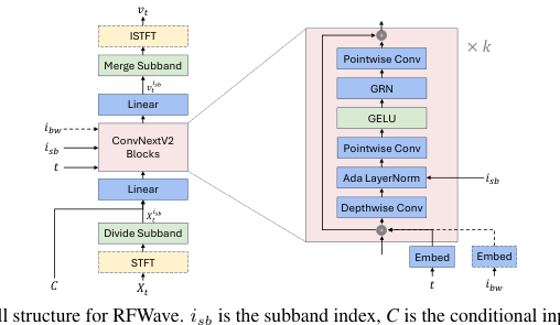Figure 1. The overall structure for RFWave. isb is the subband index, C is the conditional input, which can be an Encodec token or Mel-spectrogram, and ibw is the EnCodec bandwidth index. Modules enclosed in a dashed box, as well as dashed arrows, are considered optional

The model maps a noisy sample (Xt) to its velocity (vt). For each subband, the subband's noisy sample (Xsb) is fed into the ConvNeXtV2 backbone to predict its velocity (vs) conditioned on time (t), the subband index (ist), the conditional input (C', the Mel-spectrogram or the EnCodec (Défossez et al., 2022) tokens), and an optional EnCodec bandwidth index (ibw). The detailed structure of the ConvNeXtV2 backbone is shown in Figure 1. We employ Fourier features as described in (Kingma et al., 2021). The Xsb, C, and Fourier features are concatenated along the channel dimension and then passed through a linear layer, forming the input that is fed into a series of ConvNeXtV2 blocks. The sinusoidal t embedding, along with the optional ibw embedding, are element-wise added to the input of each ConvNeXtV2 block. The ibw is utilized during the decoding of EnCodec tokens, enabling a single model to support EnCodec tokens with various bandwidths. Furthermore, the ist is incorporated via an adaptive layer normalization module, which utilizes learnable embeddings as described in (Siuzdak, 2023; Xu et al., 2019). The other components are identical to those within the ConvNeXtV2 architecture, details can be found in (Woo et al., 2023).

Our methodology offers two modeling options. The first involves mapping Gaussian noise to the waveform directly in the time domain, wherein X0, X1, Xt and vt all reside in the time domain. The second option maps Gaussian noise to the complex spectrogram, placing X0, X1, Xt and vt in the frequency domain. Notably, Xish and vist are consistently represented in the frequency domain, as detailed in the following paragraphs, ensuring that the neural network runs at the frame level. By processing frame-level features, our model achieves greater memory efficiency compared to diffusion vocoders like PriorGrad, which operate at the level of waveform sample points. While PriorGrad (gil Lee et al., 2022) can train on 6-second² audio clips at 44.1 kHz within 30 GB of GPU memory, our model is capable of handling 177-second clips with the same memory resources.

Operating with Xt in the Time Domain and Waveform Equalization Since our model is designed to function at the frame level, when Xt and vt are in the time domain (specially, X₁ is the waveform and Xo is noise of the identical shape, with Xt and vt derived from (3)), the use of STFT and ISTFT, as illustrated in Figure 1, becomes necessary. The dimension of Xt and vt adhere to [1, T]³, where T is the waveform length in sample points. After the STFT operation, we extract the subbands by equally dividing the full-band complex spectrogram, getting Xis. Each subband Xisb

Selecting Time Points for Euler Method

Liu et al. (2023) employ equal step intervals for the Euler method, as illustrated in (4). Here, we propose selecting time points for sampling based on the straightness of transport trajectories. The time points are chosen such that the increase in straightness is equal across each step. The straightness of a learned velocity field v is defined as S(v) = ∫ E || (X1 - Xo) – v(Xt, t | C) ||² dt, which describes the deviation of the velocity along the trajectory. A smaller S(v) means straighter trajectories. This approach ensures the difficulty of each Euler step remains consistent, requiring the model to take more steps in more challenging regions. Using the same number of sampling steps, this method outperforms the equal interval approach. The implementation details are provided in Appendix Section A.5, while the algorithm is presented in Appendix Section A.9.2. We refer to this approach as equal straightness.

Results, Limitations & Conclusion

Experimental Design & Baselines

To rigorously validate RFWave's performance, the authors architected a comprehensive experimental setup, pitting their model against a range of established "victim" baselines across various audio domains and input types.

For Mel-spectrogram inputs, two primary evaluation scenarios were designed:
1. Comparison with Diffusion-based Vocoders: RFWave models were trained separately on three diverse datasets: LibriTTS (for speech), MTG-Jamendo (for music), and Opencpop (for vocal music). These models were then evaluated on their respective test sets. The baselines in this category were state-of-the-art diffusion models: PriorGrad and FreGrad.
2. Comparison with GAN-based Vocoders: A RFWave model was trained on LibriTTS. Its performance was then assessed on the LibriTTS test set (in-domain) and, crucially, on the MUSDB18 dataset (out-of-domain) to test generalization and robustness. The baselines here were widely used GAN models: Vocos and BigVGAN.

For discrete EnCodec token inputs, a universal RFWave model was trained on a large-scale, mixed dataset comprising Common Voice 7.0, DNS Challenge 4, MTG-Jamendo, FSD50K, and AudioSet. This universal model was then evaluated against EnCodec and Multi-Band Diffusion (MBD) on a custom-built unified test dataset of 900 audio samples from 15 external sources, covering speech, vocals, and sound effects. This broad evaluation aimed to prove RFWave's versatility across diverse audio types.

Evaluation Metrics: Both objective and subjective measures were employed.
* Objective metrics included ViSQOL (perceptual quality, using speech-mode for 22.05/24 kHz and audio-mode for 44.1 kHz waveforms), PESQ (Perceptual Evaluation of Speech Quality), V/UV F1 (F1 score for voiced/unvoiced classification), and Periodicity (periodicity error).
* Subjective evaluation involved crowd-sourced assessments using a 5-point Mean Opinion Score (MOS) scale (1: 'poor/unnatural' to 5: 'excellent/natural'). For each comparison, 30 listeners rated 20-40 groups of audio samples, including ground truth, RFWave, and baseline models, with randomized order.

Implementation Details: The RFWave model utilized a time-domain approach by default, incorporating three enhanced loss functions (energy-balanced, overlap, and STFT loss) and a ConvNeXtV2 backbone with 8 blocks. The complex spectrogram was divided into 8 equally spanned subbands. A key architectural choice was the use of only 10 sampling steps for inference. Ablation studies were also conducted to dissect the impact of individual components, such as frequency vs. time domain modeling, the incremental addition of each loss function, the "equal straightness" sampling strategy, different backbone architectures (ResNet vs. ConvNeXtV2), and model sizes. Inference speed was benchmarked on an NVIDIA GeForce RTX 4090 GPU with a batch size of 1.

What the Evidence Proves

The empirical evidence presented in the paper provides definitive and undeniable proof of RFWave's core mechanisms working in reality, showcasing its superior performance in both audio quality and computational efficiency.

Defeating Diffusion-based Baselines:
RFWave ruthlessly outperformed its diffusion-based "victims," PriorGrad and FreGrad, across all objective and subjective metrics when reconstructing from Mel-spectrograms (Table 1). For instance, RFWave achieved an average MOS of $3.95 \pm 0.09$, significantly higher than PriorGrad's $3.75 \pm 0.09$ and FreGrad's $2.99 \pm 0.14$. Objectively, RFWave's PESQ of $4.202$ dwarfed PriorGrad's $3.612$ and FreGrad's $3.640$. The definitive evidence for this superiority lies in RFWave's ability to generate "clearer and more consistent harmonics, particularly in high-frequency ranges," as visually confirmed by spectrograms in Appendix A.6 (Figures A.3, A.4, A.5), where baselines exhibited minor discontinuities or blurred high-frequency components. This directly validates the efficacy of Rectified Flow in achieving high-quality audio with fewer sampling steps.

Challenging GAN-based Baselines:
While GANs are known for speed, RFWave demonstrated comparable in-domain quality and superior out-of-domain generalization. On the in-domain LibriTTS test set, RFWave's MOS ($3.82 \pm 0.12$) was on par with BigVGAN ($3.78 \pm 0.11$) and Vocos ($3.74 \pm 0.10$) (Table 2). However, the true triumph came in the out-of-domain MUSDB18 dataset (Table 3), where RFWave achieved an average MOS of $3.67 \pm 0.05$, significantly surpassing BigVGAN's $3.51 \pm 0.05$ and Vocos's $3.10 \pm 0.06$. The hard evidence here is the visual analysis in Figure A.7, which shows that GAN-based models like BigVGAN and Vocos tend to produce "horizontal lines in the high-frequency regions of the spectrograms," leading to a "metallic sound quality." RFWave, in stark contrast, consistently generated "clear and well-defined high-frequency harmonics," proving its robustness and generalization capabilities as a diffusion-type model.

Dominating EnCodec Token Reconstruction:
For discrete EnCodec token inputs, RFWave (with CFG2) consistently achieved optimal scores across most metrics (MOS, PESQ, V/UV F1, Periodicity) and various bandwidths, outperforming both EnCodec and MBD (Table 4). For example, at 6.0 kbps, RFWave's MOS was $3.69 \pm 0.16$ compared to EnCodec's $3.10 \pm 0.15$ and MBD's $3.43 \pm 0.15$. This demonstrates RFWave's versatility and efficiency in reconstructing high-quality audio from compressed representations.

Ablation Study Validation:
The ablation studies (Table 5) provided crucial insights into the effectiveness of RFWave's individual components:
* The time-domain model consistently outperformed its frequency-domain counterpart (e.g., PESQ $4.127$ vs $3.872$), validating the choice for better high-frequency detail preservation.
* The energy-balanced loss was shown to mitigate low-volume noise in silent regions, improving overall performance (e.g., PESQ from $4.127$ to $4.181$), proving its role in minimizing relative error.
* The overlap loss, despite a slight PESQ dip, was essential for "smooth subband transitions" and maintaining consistency, as visually confirmed by the noticeable transitions without it (Figure A.9).
* The STFT loss effectively reduced artifacts in background noise (Figure A.8), improving PESQ from $4.158$ to $4.211$, albeit with a slight trade-off in ViSQOL and periodicity due to its emphasis on magnitude.
* The equal straightness sampling strategy significantly improved performance "for free" (PESQ $4.275$, Periodicity $0.100$), proving its efficacy over equal interval steps.
* The Rectified Flow mechanism was shown to be "critical" for efficient high-quality generation, as a DDPM approach with 50 steps performed poorly (Table 6). The ConvNeXtV2 backbone also proved superior to ResNet, enhancing both efficiency and quality.

Unprecedented Computational Efficiency:
Perhaps the most striking evidence is RFWave's vastly superior computational efficiency (Table 7). It achieved an inference speed of $162.59$ times real-time (xRT) on a single NVIDIA GeForce RTX 4090 GPU with just 10 sampling steps. This is an order of magnitude faster than diffusion baselines (PriorGrad $16.67$ xRT, FreGrad $7.50$ xRT, MBD $4.82$ xRT) and more than twice as fast as BigVGAN ($72.68$ xRT). Furthermore, RFWave consumed less GPU memory ($780$ MB) than BigVGAN ($1436$ MB). This speed advantage, maintained even at higher sampling rates (e.g., $152.58$ xRT at 44.1 kHz), definitively proves that RFWave overcomes the latency barrier of diffusion models, making it practical for real-world, real-time applications.

Limitations & Future Directions

While RFWave presents a significant leap forward in audio waveform reconstruction, it's important to acknowledge its current limitations and consider avenues for future development.

One subtle limitation observed is the ViSQOL metric's bias towards GAN-based models. Although RFWave often achieves higher MOS and other objective scores, ViSQOL sometimes favors GANs, which might not fully reflect human perceptual quality. This suggests that current objective metrics may not perfectly capture all nuances of audio quality, especially for novel generative approaches. Another interesting trade-off was seen with the STFT loss: while it effectively reduces artifacts, it can slightly degrade ViSQOL and periodicity due to its emphasis on magnitude over phase. This highlights a challenge in balancing different aspects of audio fidelity. Furthermore, while RFWave demonstrates strong out-of-domain generalization compared to GANs, the ultimate goal of a truly universal vocoder implies handling an even broader spectrum of unseen audio conditions and characteristics, which remains a continuous challenge. The computational resources required for training, particularly for the large-scale EnCodec mixed dataset (e.g., 4x A100 GPUs for 10 days), also represent a practical barrier for smaller research groups or individual developers.

Looking ahead, several exciting discussion topics emerge for further developing and evolving these findings:

• Adaptive Loss Function Design: Given the STFT loss trade-off, could we explore dynamic or context-aware weighting for the loss functions? For example, an adaptive mechanism that prioritizes phase information in certain frequency bands or during specific audio events might yield even better perceptual quality without reintroducing artifacts. This could involve learned weighting coefficients or a multi-objective optimization framework.
• Beyond Equal Straightness Sampling: The "equal straightness" method is a clever heuristic, but what if the optimal sampling trajectory isn't strictly "equally straight" in all regions of the latent space? Future work could investigate more advanced adaptive ODE solvers or reinforcement learning approaches to discover optimal, non-uniform sampling schedules that further minimize steps while maximizing fidelity, potentially even tailoring the schedule to specific audio characteristics.
• Enhanced Generalization for Extreme Out-of-Distribution Data: While RFWave excels, real-world audio is incredibly diverse and often noisy. How can we make these models even more robust to highly corrupted, extremely low-resource, or entirely novel audio types? This might involve meta-learning for rapid adaptation, self-supervised learning on vast unlabeled audio, or incorporating explicit noise modeling capabilities.
• Real-time Deployment on Constrained Hardware: Achieving 160x real-time on a high-end GPU is fantastic, but for ubiquitous applications on mobile devices or embedded systems, further optimizations are needed. This could involve exploring model quantization, pruning, knowledge distillation, or designing specialized architectures that are inherently more efficient on edge hardware, pushing the boundaries of what's possible in real-time audio synthesis.
• Multi-modal and Interactive Audio Generation: The current work focuses on Mel-spectrograms and discrete tokens. Expanding RFWave to directly incorporate other modalities like text, video, or even user-defined parameters (e.g., emotional cues, spatial audio properties) could unlock new creative applications and more intuitive human-computer interaction. Imagine generating audio that perfectly matches a video scene's mood or a user's gestural input.
• Development of Perceptually Aligned Metrics: The observed ViSQOL bias underscores a broader need in the field. How can we develop new objective metrics that are more robust, less biased, and more closely align with human perception of "naturalness" and "quality" in synthetic audio, especially as models generate increasingly complex and novel sounds? This could involve leveraging human-in-the-loop feedback or advanced psychoacoustic modeling.
• Ethical Implications and Safeguards: As audio synthesis becomes indistinguishable from real recordings, the ethical implications, such as the creation of deepfakes or misuse in misinformation, grow. Future research should proactively address these concerns by exploring methods for watermarking synthetic audio, developing robust detection mechanisms, or integrating ethical guidelines directly into the model design and deployment process. This is a crucial, often overlooked, aspect of advancing generative AI.