Adaptive Stain Normalization for Cross-Domain Medical Histology

Background & Academic Lineage

The Origin & Academic Lineage

The problem addressed in this paper originates from the critical role of pathological examination in disease diagnosis, which traditionally relies on manual assessment of digital pathology images. While manual review provides crucial insights into tissue morphology and cellular abnormalities, it is inherently labor-intensive, time-consuming, and prone to variability between different observers [20,19]. The advent of deep learning offered a promising path towards automating this analysis, but it quickly encountered a significant hurdle: color inconsistency in digital pathology images.

This color variability, a major challenge for model generalizability, stems from several factors: (i) differences in chemical reactions and exposure times of dyes during the staining process, (ii) variations in sample preparation, and (iii) diverse imaging conditions across different scanning hardware [15]. While experienced human pathologists can intuitively compensate for these variations, deep learning models are highly sensitive to such "domain shifts," leading to a significant drop in performance and poor generalization when applied to data acquired under different conditions than their training data [3]. This "pain point" forced the academic field, particularly in medical pathology, to develop strategies for stain color normalization to ensure consistent image appearance across diverse datasets.

Previous approaches to stain normalization, while attempting to mitigate these issues, suffered from several fundamental limitations. Traditional methods often required the careful selection of a "template" image from the training domain to match color statistics, which demanded prior knowledge and could introduce artifacts. Physics-based methods, such as those leveraging the Beer-Lambert law and Nonnegative Matrix Factorization (NMF), improved upon this by accounting for the underlying image formation process. However, they still typically relied on predefined templates or required additional prior knowledge, such as the absorption spectrum matrix of specific dyes or the exact number of distinct color components [18]. Furthermore, the use of Principal Component Analysis (PCA) in some NMF-based methods had deficiencies, as it assumes orthogonal components, which is not always realistic for stain components. More recent deep learning-based methods, like Generative Adversarial Networks (GANs), could align color distributions but often introduced synthetic artifacts or "hallucinated" cellular structures, posing risks in medical diagnosis [12]. Other deep learning techniques were often too generic, failing to account for the specific physics of histological staining [10]. The authors of this paper sought to overcome these limitations by proposing a trainable, physics-informed, and template-free solution that could adaptively disentangle stain information.

Intuitive Domain Terms

1. Domain Shift: Imagine you've trained a dog to recognize a red ball. If you then show it a blue ball, it might get confused because the "domain" (the color of the ball) has shifted. In digital pathology, it means a deep learning model trained on images from one lab (with specific staining and imaging) might perform poorly on images from another lab with slightly different conditions.
2. Stain Normalization: Think of it like using a photo filter to make all your pictures have the same consistent look, even if they were taken in different lighting. In histology, it's a process to adjust the colors of tissue slides so that they all appear as if they were stained using the exact same protocol, making them comparable for automated analysis.
3. Beer-Lambert Law: This is a basic rule in optics, like how a pair of sunglasses works. It tells you how much light passes through a material (like stained tissue) based on how thick the material is and how much of the light-absorbing substance (the stain) is present. It's crucial for understanding how stains give tissue its characteristic color.
4. Nonnegative Matrix Factorization (NMF): Picture a fruit salad where you want to figure out exactly what fruits were used and in what quantities, knowing you can't have "negative" amounts of any fruit. NMF is a mathematical technique that breaks down a complex image (like a stained tissue slide) into its fundamental, non-negative components, such as the individual stains and their concentrations at each pixel.
5. Algorithmic Unrolling: Consider a complex iterative calculation, like repeatedly adjusting a telescope's focus until the image is sharp. "Unrolling" means taking each step of that iterative process and turning it into a distinct layer within a neural network. This allows the entire sequence of adjustments to be learned and optimized end-to-end, rather than being a fixed, separate process.

Notation Table

Notation	Description

Problem Definition & Constraints

Core Problem Formulation & The Dilemma

The central problem this paper addresses stems from the inherent color variability in digital pathology images, a critical issue for the reliability and generalizability of deep learning models in medical diagnosis.

Input/Current State: The input is a digital pathology image, represented as $X \in \mathbb{R}^{c \times p}$, where $c$ is the number of color intensities (typically 3 for RGB) and $p$ is the number of pixels. This image $X$ exhibits significant color inconsistencies due to various factors: differences in staining protocols, chemical reactions, dye exposure times, sample preparation variability, and diverse imaging conditions across different scanning hardware. This color inconsistency leads to a "domain shift," meaning deep learning models trained on data from one set of conditions perform poorly when applied to data from another.

Desired Endpoint/Goal State: The desired output is a "stain-normalized" image or, more precisely, a "stain-invariant structural information" representation derived from the input image. This normalized representation should effectively remove color variability while preserving the underlying tissue morphology and cellular abnormalities. The ultimate goal is to feed this robust, stain-invariant representation into downstream deep learning tasks, such as object detection and image classification, enabling these models to generalize effectively across different domains and achieve consistent, high performance regardless of the original image's staining appearance.

Missing Link/Mathematical Gap: The exact missing link is a robust, adaptive, and physics-informed method to mathematically disentangle the stain information from the structural content of the image. Previous approaches, motivated by the Beer-Lambert law, model the image intensity $X$ as a function of incident light $x_0$, a color appearance matrix $S$, and an optical density matrix $D$:
$$X = (x_0 \mathbf{1}^T) \odot e^{-SD^T}$$
where $\mathbf{1}$ is a vector of all ones and $\odot$ denotes element-wise matrix product. The mathematical gap lies in reliably estimating $x_0$, $S$, and $D$ from a given input image $X$ in a way that is:
1. Adaptive: Does not require prior knowledge of staining protocols or template images.
2. Physics-informed: Respects the non-negativity of color spectra and optical densities.
3. Trainable: Can be integrated end-to-end with deep learning architectures.
4. Structure-preserving: Avoids introducing synthetic artifacts.

The paper aims to bridge this gap by refining existing Non-negative Matrix Factorization (NMF) models, which are often non-convex and require careful parameter tuning, into a trainable, unrolled network architecture.

The Dilemma: Previous researchers have been trapped by several painful trade-offs:
* Template Dependency vs. Adaptability: Many existing stain normalization methods rely heavily on a "template image" or require a priori knowledge (e.g., absorption spectra of specific dyes, number of color components). While these methods can be effective for specific, well-defined domains, they fail to adapt to new or arbitrary staining protocols without manual intervention or careful template selection, severely limiting their generalizability.
* Physics-Informed Accuracy vs. Artifact Generation: Methods that strictly adhere to the physics of staining (like those based on the Beer-Lambert law and NMF) often employ heuristics (e.g., Principal Component Analysis for $S$ and $D$) that introduce deficiencies, such as requiring orthogonality which is unrealistic for stain components. Conversely, more generic deep learning approaches, like Generative Adversarial Networks (GANs), can align color distributions but are prone to "hallucinating" cellular structures or introducing synthetic artifacts, which is unacceptable and dangerous in medical diagnostics.
* Fixed Parameters vs. Learnability: Earlier NMF models (e.g., Equation 3) require manual tuning of parameters like the sparse regularization strength $\lambda$ and the rank $r$ (number of colored components). This manual tuning is challenging, especially when the number of colored components is unknown, and prevents seamless integration into end-to-end deep learning pipelines where parameters are learned automatically.

Constraints & Failure Modes

The problem of adaptive stain normalization is insanely difficult due to several harsh, realistic walls the authors hit:

• Physical Constraints:

  • Beer-Lambert Law Adherence: Any effective model must accurately represent the physical process of light attenuation by stains. This means respecting the multiplicative nature of light absorption and the decomposition into stain concentrations and absorption properties.
  • Non-negativity: Both the color spectra ($S$) and optical densities ($D$) are physically non-negative quantities. Enforcing this constraint is crucial for a meaningful decomposition, but it adds complexity to optimization problems.
  • Stain-Invariant Information: The core challenge is to extract structural information that is truly independent of the staining appearance. This requires a robust separation of color information from morphological details, which is not trivial given their intertwined nature in raw images.

• Computational Constraints:

  • Non-convex Optimization: The underlying NMF problem, particularly with the $SD^T$ matrix product, is non-convex. This means standard optimization algorithms can get stuck in local minima, making it hard to find globally optimal solutions.
  • End-to-End Trainability: For practical deployment with modern deep learning models, the stain normalization process must be differentiable and capable of being trained end-to-end. Many traditional methods involve non-differentiable steps or heuristics, preventing their seamless integration into deep learning frameworks.
  • Computational Efficiency: Processing large whole slide images in real-time or near real-time for clinical applications demands computationally efficient algorithms. Complex iterative optimization procedures can be prohibitively slow.

• Data-Driven Constraints:

  • Extreme Domain Shift: Digital pathology datasets exhibit significant color variability not just between different labs or scanners, but even within the same lab over time. This "domain shift" is a primary cause of deep learning model failure, requiring a normalization method that can handle large and unpredictable variations.
  • Lack of Prior Knowledge: In many real-world scenarios, detailed a priori knowledge about the specific staining protocols, dye absorption spectra, or the exact number of colored components in a specimen is unavailable. A robust method must operate effectively without such explicit inputs.
  • Artifact Avoidance: Unlike general image style transfer, medical image analysis cannot tolerate the introduction of "synthetic artifacts" or "hallucinated" structures during normalization. Such distortions could lead to misdiagnosis, making structure preservation a paramount constraint.

• Failure Modes of Previous Approaches (which become constraints for a new solution):

  • Template-induced Bias: Relying on a fixed template image can introduce bias and limit adaptability, as the chosen template might not be representative of all target domains.
  • Parameter Sensitivity: Previous NMF models required careful, manual selection of regularization parameters and the number of components ($r$), which is often a trial-and-error process and can lead to suboptimal results if not chosen correctly.
  • Orthogonality Assumption: Methods like PCA, used in some prior works to estimate stain components, impose an orthogonality constraint that is not physically realistic for biological stains, leading to inaccurate decompositions.
  • Permutation Ambiguity: The decomposition of $S$ and $D$ can suffer from permutation ambiguity, where columns might be swapped, leading to "significant color distortions" if not handled correctly.

Why This Approach

The Inevitability of the Choice

The development of BeerLaNet was driven by the clear and persistent shortcomings of existing stain normalization methods when confronted with the complex realities of digital pathology. The core problem, as highlighted in the paper, is the "domain shift" caused by significant color variability due to differences in staining protocols and imaging conditions. This variability severely degrades the perfomance of deep learning models, hindering their generalizability.

Traditional stain normalization techniques, such as those relying on statistical matching or color space decomposition (e.g., Reinhard, Macenko, Vahadane), were found to be insufficient primarily becuase they depend heavily on "appropriate representative templates" or "prior knowledge of the domain." This often includes requiring specific dye absorption spectra or a predefined number of color components. Such dependencies make these methods brittle and prone to "significant color distortions" when the template is poorly chosen or when faced with unknown staining protocols. The authors realized that a method requiring such explicit prior knowledge or careful manual selection of templates and parameters could not be the only viable solution for a truly adaptive and robust system.

Deep learning-based alternatives, like Generative Adversarial Networks (GANs) for style transfer (e.g., StainGAN), also presented critical flaws. While capable of aligning color distributions, GANs often "introduce synthetic artifacts or 'hallucinate' cellular structures," which poses unacceptable risks in medical diagnosis where fidelity to the original morphology is paramount. Other deep learning methods using attention mechanisms were deemed "largely generic" and failed to account for the underlying physics of image formation, limiting their robustness and interpretability.

The exact moment the authors realized these SOTA methods were insufficient was when they observed that the existing physics-informed matrix factorization models, while conceptually sound, suffered from practical limitations. Specifically, the sparse Non-negative Matrix Factorization (NMF) model in equation (3) was non-convex and required a priori specification of the number of colored components ($r$), a challenging task when this number is unknown (e.g., when specimens contain additional colored components like hemoglobin). Furthermore, the use of Principal Component Analysis (PCA) in earlier physics-based models was problematic as it assumes orthogonal columns, which is unrealistic for stain separation. This confluence of issues—template dependency, artifact generation, lack of physics-informed adaptability, and fixed parameter requirements—made it clear that a fundamentally new, integrated approach was necessary.

Comparative Superiority

BeerLaNet achieves qualitative superiority over previous gold standards through several structural advantages that go beyond mere performance metrics. Firstly, its Adaptive Stain Disentanglement allows it to extend to "arbitrary staining protocols," learning "stain-invariant representations of images without requiring any prior knowledge of the staining protocol." This is a profound advantage over template-based methods that are inherently limited by the quality and representativeness of their chosen templates. BeerLaNet's ability to operate template-free and without prior knowledge of specific dyes or components makes it far more robust and generalizable across diverse clinical settings.

Secondly, the method is Trainable and Physics-Informed, built upon Non-negative Matrix Factorization (NMF) and algorithmic unrolling. This combination is a key structural innovation. By deriving the model architecture via algorithmic unrolling of a modified NMF formulation (equation 4), BeerLaNet transforms a traditionally non-convex optimization problem into an end-to-end trainable deep network. This allows for the learnable adaptation of regularization parameters ($\gamma, \lambda$) and initializations ($S_{init}$), which were previously fixed or heuristically chosen. This data-driven learning, grounded in the Beer-Lambert law, ensures that the stain decomposition process is both physically accurate and highly adaptable, avoiding the pitfalls of generic color transformations that disregard the underlying imaging physics.

The incorporation of an additional $l_2$ regularization in the modified NMF formulation (4) is another structural advantage. This regularization promotes low-rank solutions, enabling the model to initialize the number of colored components ($r$) larger than expected and then adapt the rank of the solution to the data. This elegantly solves the problem of a priori specification of $r$, making the model more flexible and robust to variations in specimen composition.

Finally, BeerLaNet's Flexible Integration as a plug-and-play module means it can be seamlessly combined with any backbone network for downstream tasks. This architectural design ensures that the stain normalization is not a standalone preprocessing step but an integral, learnable part of the entire deep learning pipeline, optimizing the normalization specifically for the end task (e.g., object detection or classification). This end-to-end trainability is a significant structural advantage over methods that operate in isolation and cannot adapt their normalization process based on downstream task feedback.

Alignment with Constraints

BeerLaNet's design perfectly aligns with the harsh requirements of stain normalization in medical histology, forming a strong "marriage" between problem and solution.

1. Constraint: Overcome Color Inconsistency and Domain Shift: The primary goal is to generalize across varying staining and imaging conditions. BeerLaNet addresses this through its "Adaptive Stain Disentanglement," which learns "stain-invariant representations" without needing prior knowledge of the staining protocol. This directly tackles the root cause of domain shift by extracting the underlying biological information independent of color variations.

2. Constraint: Avoid Artifacts and Hallucinations: Crucial for medical diagnosis. BeerLaNet achieves this by being "Physics-Informed." Its foundation in the Beer-Lambert law ensures that the stain decomposition is grounded in the actual light-tissue interaction, making the transformations physically plausible and less likely to introduce synthetic artifacts compared to purely data-driven, generic deep learning models like GANs.

3. Constraint: Eliminate Template Dependency and Prior Knowledge: Traditional methods struggled with requiring specific templates or a priori knowledge (e.g., absorption spectra, number of components). BeerLaNet's "Trainable and Physics-Informed" nature, coupled with algorithmic unrolling, allows it to learn these parameters from data. The $l_2$ regularization enables the model to adapt the number of components ($r$) to the data, removing the need for manual specification. This makes the method entirely template-free and independent of explicit prior knowledge.

4. Constraint: Support Diverse Staining Protocols: Many previous methods focused primarily on H&E stains. BeerLaNet explicitly "extends to arbitrary staining protocols," making it a more universally applicable solution for the wide variety of stains used in pathology.

5. Constraint: Seamless Integration with Downstream Tasks: The solution must be practical for real-world diagnostic pipelines. BeerLaNet is designed as a "Flexible Integration" module, a "plug-and-play" component that can be combined with "arbitrary backbone networks for downstream tasks such as object detection and classification." This ensures that the normalization process is optimized within the context of the final diagnostic task, enhancing overall system performance.

Rejection of Alternatives

The paper provides clear reasoning for rejecting alternative approaches, both traditional and deep learning-based.

Traditional Methods (e.g., Reinhard, Macenko, Vahadane): These methods were rejected primarily due to their inherent reliance on template images and prior knowledge. As stated, they "strongly relies on selecting appropriate representative templates" and "can require prior knowledge of the domain," such as the absorption spectrum matrix of specific dyes or the number of distinct color components. This dependency makes them brittle; if the template is not representative or the prior knowledge is inaccurate, these methods can lead to "significant color distortions." Furthermore, they often require careful manual selection of parameters like regularization strength ($\lambda$) and the rank of the matrix factorization ($r$). The experimental results in Table 1 quantitatively support this rejection, showing that these methods often exhibit a "large drop in performance" on datasets with greater domain variations, such as the malaria dataset, indicating poor generalization.

Deep Learning-based Methods (e.g., StainGAN, LStainNorm):
* GANs (e.g., StainGAN): These were rejected due to a critical flaw for medical applications: they "can often introduce synthetic artifacts or 'hallucinate' cellular structures, posing risks in medical diagnosis [12]." In a field where diagnostic accuracy and fidelity to biological reality are paramount, any method that compromises image integrity is unacceptable.
* Attention Mechanisms (e.g., LStainNorm): These methods were deemed "largely generic and do not necessarily account for the relevant image formation process [10]." This implies a lack of grounding in the underlying physics of staining, which can limit their robustness and interpretability compared to BeerLaNet's physics-informed approach.

The experimental results further validate these rejections. The paper notes that "Methods with a generic design that do not incorporate stain-specific characteristics may perform well on small domain shift data (Camelyon17-WILDS, whole blood cells) but fail to generalize to the large color shifts observed in the malaria dataset." This directly contrasts with BeerLaNet's consistent and superior performance across diverse tasks and datasets, especially those with significant domain shifts, underscoring the limitations of the alternatives in real-world, challenging scenarios.

Mathematical & Logical Mechanism

The Master Equation

The core of the BeerLaNet method, which drives its stain normalization capabilities, is an optimization problem derived from a sparse Non-negative Matrix Factorization (NMF) model. This model is itself rooted in the Beer-Lambert law, which describes how light is attenuated by stains. The specific objective function that BeerLaNet unrolls and optimizes is given by:

$$ \min_{x_0,S,D} \frac{1}{2} ||x_0\mathbf{1}^T - X - SD^T||_F^2 + \lambda \sum_{i=1}^r (||s_i||_2^2 + ||d_i||_1 + ||d_i||_2^2) \text{ s.t. } S,D \ge 0. $$

This equation seeks to find the optimal background light intensity ($x_0$), stain color profiles ($S$), and stain concentrations ($D$) that best explain the input image, while also promoting desirable properties like sparsity and low-rank solutions.

Term-by-Term Autopsy

Let's dissect this master equation to understand the role of each component:

• $X$: This is the input image matrix, typically of size $C \times P$, where $C$ is the number of color channels (e.g., 3 for RGB) and $P$ is the total number of pixels. Each column of $X$ represents the color intensities for a single pixel. Crucially, given the derivation from the Beer-Lambert law's logarithmic form (Equation 2 in the paper), this $X$ implicitly represents the element-wise logarithm of the observed image intensities.

  • Mathematical Definition: A $C \times P$ matrix representing the logarithmic color intensities of the input image.
  • Physical/Logical Role: It's the raw, observed data that the model attempts to decompose. The goal is to explain this observed image as a combination of background light and stain effects.
  • Why used: It's the direct representation of the image data in a format suitable for matrix factorization.

• $x_0$: This is a vector in $\mathbb{R}^C$ representing the incident light intensity or background illumination.

  • Mathematical Definition: A $C$-dimensional vector.
  • Physical/Logical Role: In the context of the Beer-Lambert law, $x_0$ models the light source's intensity before it interacts with the stained tissue. It accounts for variations in illumination conditions.
  • Why used: It's a fundamental component of the Beer-Lambert law, allowing the model to adapt to different lighting scenarios.

• $\mathbf{1}^T$: This is a row vector of all ones, with dimensions $1 \times P$.

  • Mathematical Definition: A $1 \times P$ matrix where all elements are 1.
  • Physical/Logical Role: When multiplied with $x_0$, it effectively broadcasts the background light intensity $x_0$ to all pixels, creating a matrix where every pixel is assumed to be illuminated by $x_0$.
  • Why used: To apply the background light intensity uniformly across all pixels for matrix operations.

• $x_0\mathbf{1}^T$: This term represents the incident light matrix across all pixels.

  • Mathematical Definition: A $C \times P$ matrix where every column is the vector $x_0$.
  • Physical/Logical Role: It's the "unattenuated" light matrix, representing the light that would be observed if there were no stains.
  • Why used: It forms the baseline from which stain-induced attenuation is subtracted, as per the logarithmic Beer-Lambert law.

• $S$: This is the color appearance matrix, of size $C \times r$, where $r$ is the number of colored components. Each column $s_i \in \mathbb{R}^C$ represents the color spectrum (absorption characteristics) of the $i$-th colored component (e.g., a specific stain like hematoxylin or eosin).

  • Mathematical Definition: A $C \times r$ matrix.
  • Physical/Logical Role: This matrix captures the unique "fingerprint" of each stain, describing how it absorbs light across different color channels. It's essential for disentangling the distinct stain colors.
  • Why used: It allows the model to learn the spectral properties of stains directly from the data, without requiring prior knowledge of specific dyes.

• $D$: This is the optical density matrix, of size $P \times r$. Each column $d_i \in \mathbb{R}^P$ contains the optical density (concentration) of the $i$-th colored component at each pixel.

  • Mathematical Definition: A $P \times r$ matrix.
  • Physical/Logical Role: This matrix represents the spatial distribution and concentration of each stain component across the image. It's the "stain-invariant structural information" that BeerLaNet aims to extract, as it describes where and how much of each stain is present, independent of its color.
  • Why used: It's the other core component of the Beer-Lambert law, representing the amount of each stain present at each pixel.

• $SD^T$: This matrix product, of size $C \times P$, represents the total optical density contribution from all stains across all pixels, transformed back into the color space.

  • Mathematical Definition: A $C \times P$ matrix resulting from the product of $S$ and $D^T$.
  • Physical/Logical Role: In the logarithmic Beer-Lambert law, this term represents the total attenuation caused by the stains. It's the "stain effect" that needs to be modeled and, subsequently, removed for normalization.
  • Why used: It's the mathematical representation of how the stain color profiles ($S$) are distributed ($D$) to cause light attenuation.

• $||x_0\mathbf{1}^T - X - SD^T||_F^2$: This is the data fidelity term, specifically the squared Frobenius norm of the residual matrix.

  • Mathematical Definition: The sum of the squares of all elements in the matrix $(x_0\mathbf{1}^T - X - SD^T)$.
  • Physical/Logical Role: This term measures how well the model's reconstruction of the image (based on $x_0, S, D$) matches the actual input image $X$. Minimizing this term means the model is trying to find $x_0, S, D$ such that their combination accurately explains the observed image.
  • Why used: The squared Frobenius norm is a standard and differentiable way to quantify the difference between matrices, making it suitable for gradient-based optimization. The $\frac{1}{2}$ factor is a common convention to simplify its derivative.

• $\lambda$: This is a non-negative scalar regularization paramter.

  • Mathematical Definition: A scalar value.
  • Physical/Logical Role: It controls the strength of the regularization terms. A larger $\lambda$ places more emphasis on promoting sparsity and low-rank properties in $S$ and $D$, potentially at the expense of perfect data reconstruction. It acts as a balancing knob.
  • Why used: To prevent overfitting and encourage the learned stain components to have desirable mathematical properties, and it's made learnable in BeerLaNet.

• $\sum_{i=1}^r (\dots)$: This denotes a summation over the $r$ colored components.

  • Mathematical Definition: A sum from $i=1$ to $r$.
  • Physical/Logical Role: It aggregates the regularization penalties for each individual stain component ($s_i$ and $d_i$) into a single total penalty.
  • Why used: To apply the regularization uniformly to all identified stain components.

• $||s_i||_2^2$: This is the squared L2 norm of the $i$-th column of $S$.

  • Mathematical Definition: The sum of the squares of the elements in the vector $s_i$.
  • Physical/Logical Role: This term regularizes the magnitude of the color spectra vectors. It encourages the elements of $s_i$ to be small, preventing any single color channel from having an excessively large contribution to a stain's profile. It also promotes low-rank solutions for $S$.
  • Why used: It helps in finding a more compact and meaningful set of stain components, as mentioned in the paper, by promoting low-rank solutions.

• $||d_i||_1$: This is the L1 norm of the $i$-th column of $D$.

  • Mathematical Definition: The sum of the absolute values of the elements in the vector $d_i$.
  • Physical/Logical Role: This term promotes sparsity in the optical density matrix $D$. It encourages many elements of $d_i$ to be exactly zero, meaning that a particular stain component is present only in a few pixels. This aligns with the assumption that "relevant histological features of interest are sparse in space."
  • Why used: L1 regularization is a standard technique for inducing sparsity, which helps to isolate distinct stain regions and makes the interpretation of $D$ more meaningful.

• $||d_i||_2^2$: This is the squared L2 norm of the $i$-th column of $D$.

  • Mathematical Definition: The sum of the squares of the elements in the vector $d_i$.
  • Physical/Logical Role: Similar to $||s_i||_2^2$, this term regularizes the magnitude of the optical density vectors. It prevents any single pixel from having an excessively high concentration of a stain and contributes to promoting low-rank solutions for $D$.
  • Why used: For promoting low-rank solutions and preventing overly large values in $D$, contributing to numerical stability and better generalization.

• $\text{s.t. } S,D \ge 0$: These are non-negativity constraints.

  • Mathematical Definition: All elements in matrices $S$ and $D$ must be greater than or equal to zero.
  • Physical/Logical Role: This is a crucial physical constraint. Stain concentrations (optical densities in $D$) and light absorption coefficients (in $S$) cannot be negative. Negative values would be physically meaningless. This is a defining characteristic of Non-negative Matrix Factorization (NMF).
  • Why used: To ensure that the learned stain components and their concentrations are physically interpretable and adhere to the underlying Beer-Lambert law, which is based on non-negative quantities.

The choice of addition for combining the data fidelity and regularization terms is standard in optimization, allowing for a balance between fitting the data and promoting desired properties. Summations are used instead of integrals because the problem deals with discrete entities: pixels, color channels, and stain components.

Step-by-Step Flow

BeerLaNet operates by "unrolling" the optimization process of the master equation into a series of iterative steps, much like an assembly line. Let's trace how an abstract data point (a single pixel's color vector $x_j$ from the input image $X$) would flow through this mechanism for one iteration $k$:

1. Input Entry: An entire input image $X$ (a $C \times P$ matrix) is fed into the BeerLaNet module. At this stage, we have initial or previous estimates for the background light $x_0^{(k-1)}$, the stain color matrix $S^{(k-1)}$, and the optical density matrix $D^{(k-1)}$.
2. Background Light Update ($x_0$): The first station on our assembly line updates the background light $x_0$. Each pixel's color vector $x_j$ (from $X$) is conceptually combined with the current estimate of its stain contribution (derived from $S^{(k-1)}$ and $D^{(k-1)}$). These combined values are then averaged across all pixels to produce a new, refined estimate for $x_0^{(k)}$. This step essentially determines the overall incident light that, when attenuated by the current stain model, best reconstructs the observed image.
3. Optical Density Update ($D$): Next, the system focuses on updating the optical density matrix $D$.
   • Step Size Calculation: A dynamic step size $\tau_D$ is calculated, which dictates how aggressively $D$ should be updated in this iteration.
   • Gradient Descent: For each pixel, its current stain concentrations (represented by a row in $D^{(k-1)}$) are adjusted. This adjustment is based on how well the current $S$ and $D$ explain the input image $X$ and the newly updated $x_0^{(k)}$. The gradient pushes $D$ towards values that minimize the reconstruction error.
   • Proximal Operators (Sparsity & Non-negativity): After the gradient step, a series of "clipping" and "shrinking" operations are applied to each column $d_i$ of $D$. These are the proximal operators. They enforce two critical properties:
     • Non-negativity: Any negative concentration values are immediately clipped to zero, ensuring physical realism.
     • Sparsity: The L1 norm regularization encourages many concentration values to become exactly zero. This means that for a given pixel, if a stain component's concentration is very low, it's effectively removed, making the representation sparse and highlighting only the dominant stains.
     • L2 Regularization: An additional L2 proximal operator further regularizes the magnitude of $d_i$, preventing excessively high concentrations and promoting low-rank solutions.
   • Analyst's Note: To be honest, I’m not completely sure about the exact form of the proximal operators for $D$ and $S$ as described in Algorithm 1 (lines 10 and 17). The terms like $\lambda\gamma\tau||s_i||_2^2$ or $\lambda\gamma\tau_S(d_1+d_2)$ are not standard for the L1 or L2 proximal operators of the objective function (4) and seem to contain a slight discrepency or a highly specialized formulation not fully detailed in the text. However, the intent is clearly to enforce non-negativity, sparsity (for $D$), and magnitude regularization (for both $S$ and $D$).
4. Stain Color Update ($S$): The process then moves to update the stain color matrix $S$.
   • Step Size Calculation: A dynamic step size $\tau_S$ is computed for $S$.
   • Gradient Descent: Each stain's color profile (a column in $S^{(k-1)}$) is adjusted based on how well the current $S$ and the newly updated $D^{(k)}$ explain the image $X$ and background $x_0^{(k)}$. This refines the spectral characteristics of each stain.
   • Proximal Operators (Magnitude & Non-negativity): Similar to $D$, proximal operators are applied to each column $s_i$ of $S$:
     • Non-negativity: Ensures that absorption coefficients are physically meaningful (non-negative).
     • L2 Regularization: Scales down the magnitude of the color vectors, contributing to the low-rank property of $S$ and preventing any single color channel from having an overly dominant spectral contribution.
5. Iteration End: This completes one unrolled iteration. The refined $x_0^{(k)}, S^{(k)}, D^{(k)}$ are now ready for the next iteration, or if $K$ iterations are complete, for the final output.
6. Output & Downstream Integration: After $K$ iterations, the final $D$ matrix, representing the stain-invariant structural information, is extracted. This $P \times r$ matrix is then reshaped into an $r$-channel image (where each channel corresponds to the spatial distribution of one stain component). This $r$-channel image is then passed through a $1 \times 1$ convolution layer to map it back to a 3-channel image, which can then be seamlessly integrated into any deep learning backbone network (like YOLO or ResNet) for downstream tasks such as object detection or classification.
   An overview of our approach is depicted in Fig. 1, and the full details of our method are given in Algorithm 1.

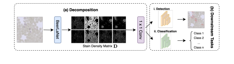Figure 1. Overview of our proposed BeerLaNet method

Optimization Dynamics

The mechanism by which BeerLaNet "learns" and converges is through an unrolled alternating proximal gradient descent algorithm, which is then trained end-to-end.

• Alternating Proximal Gradient Descent: The core optimization strategy is iterative. It tackles the non-convex objective function by alternately optimizing one set of paramters ($x_0$, then $D$, then $S$) while keeping the others fixed. For each variable, it combines a standard gradient descent step (to minimize the smooth data fidelity term) with a proximal operator (to handle the non-smooth regularization terms and non-negativity constraints). This iterative refinement helps the model navigate the complex loss landscape.
• Non-convex Loss Landscape: The presence of the $SD^T$ product makes the objective function non-convex. This means the loss landscape is not a simple bowl shape; it can have multiple "valleys" or local minima. While alternating proximal gradient descent is effective, it doesn't guarantee finding the absolute best (global) minimum. However, in practice, it often finds good solutions.
• Gradients and Updates: During the gradient descent phases for $D$ and $S$, the algorithm calculates the gradients of the data fidelity term. These gradients point in the direction where the reconstruction error increases most steeply. The algorithm then takes a step in the opposite direction, iteratively reducing this error. The dynamic step sizes ($\tau_D, \tau_S$) are crucial; they adapt to the local curvature of the loss landscape, allowing for larger steps when the landscape is flat and smaller steps when it's steep, aiding in faster and more stable convergence.
• Proximal Operators' Role: The proximal operators are vital for shaping the solution. For $D$, the L1 norm encourages sparsity, effectively setting small stain concentrations to zero, which simplifies the stain map. For both $S$ and $D$, the L2 norms and non-negativity constraints ensure that the learned stain profiles and concentrations are physically meaningful and well-behaved, preventing unrealistic values or overfitting.
• Learnable Parameters and End-to-End Training: A key innovation of BeerLaNet is making some critical optimization hyperparameters (like $\lambda$, $\gamma$, and the initial $S_{init}$) learnable. Instead of manually tuning these, the entire unrolled optimization process is embedded within a neural network architecture. The loss from the final downstream task (e.g., object detection accuracy) is then backpropagated through all $K$ unrolled layers. This means that the gradients flow all the way back to update not only the weights of the downstream backbone network but also the regularization paramters and initial stain estimates within BeerLaNet. This end-to-end training allows the BeerLaNet module to adapt its internal stain normalization process to directly optimize for the performance of the final task, making it highly adaptive and robust.
• Convergence Behavior: With each unrolled iteration, the estimates of $x_0, S, D$ are progressively refined. The number of unrolled iterations, $K$, acts like the depth of the BeerLaNet module. The backpropagation through these unrolled layers guides the iterative process towards a solution that is not just optimal for the NMF objective, but specifically for the ultimate goal of the downstream task, leading to improved generalization across different stain domains.

Results, Limitations & Conclusion

Experimental Design & Baselines

To rigorously validate BeerLaNet's ability to provide adaptive stain normalization and enhance cross-domain generalization, the authors architected a comprehensive experimental setup across two primary diagnostic tasks: object detection and image classification. They pitted BeerLaNet against a suite of established baseline models, both classical and deep learning-based, across diverse pathology datasets.

For object detection, the evaluation focused on malaria parasite detection and whole blood cell detection. The malaria detection task utilized a public dataset [5] comprising 24,720 May Grunwald-Giemsa (MGG)-stained thin blood smear images, annotated for white blood cells, red blood cells, platelets, and various parasite species. A separate, internally curated test dataset of 264 thin blood smear images from a Zeiss Axioscan microscope was used for evaluation. For whole blood cell detection, two public datasets were employed: BCCD [17] for training (366 images) and BCDD [1] for testing (100 images). BeerLaNet was integrated with a YOLOv8 backbone [9] for these tasks.

For image classification, two distinct challenges were addressed: malaria parasite classification and breast cancer classification. The malaria classification dataset was a diverse collection from four microscopy platforms (Hamamatsu NanoZoomer, Zeiss Axioscan, Olympus CX43, Morphle Hemolens), featuring Giemsa-stained thin blood smears. It included a training set of 2,486 single-cell cropped images and two test sets (343 and 261 samples) from distinct imaging platforms, designed to assess generalization across domains. The task involved classifying detected parasites by lifestage. For breast cancer classification, the Camelyon17-WILDS dataset [2] was used, consisting of 96x96 image patches from lymph node whole slide images, with tumor presence labels. This dataset spanned five hospitals, inherently introducing significant domain shifts. BeerLaNet was integrated with a ResNet-18 backbone [8] for classification tasks.

The "victims" (baseline models) against which BeerLaNet was compared included three classical histology normalization methods: Reinhard [13], Macenko [11], and Vahadane [18]. Additionally, two deep learning-based methods, StainGAN [16] and LStainNorm [10], were included. For baselines requiring a template image for normalization, one image was randomly selected from the training dataset.

Key implementation details for BeerLaNet included setting the number of colored components ($r$) to 8 and internal unrolled iterations ($K$) to 10. Training parameters varied by task, with batch sizes of 8 (detection) or 128 (classification) and learning rates of 0.01 or 1e-4. Notably, a two-step denoising pipeline (median and Gaussian filters) was applied to the malaria classification dataset to mitigate compression artifacts. All experimental results were averaged across three random seeds to ensure robustness.

Evaluation metrics were chosen to reflect the specific task requirements: mAP50 and mAP50-95 for detection, and Accuracy (Acc) for classification. A specialized Relaxed Accuracy (RAcc) was introduced for malaria parasite classification, considering predictions successful if within one lifestage of the ground truth, acknowledging the continuous nature of parasite growth. To provide a definitive, undeniable measure of consistent performance across all tasks and datasets, the authors introduced the Average Percent Underperformance (APU) metric. This metric quantifies the average percent difference between a method's performance and the best-performing method for each task-metric combination, providing a holistic view of generalization.
example images showing the variance in domain between training and testing data are displayed in Fig 2.

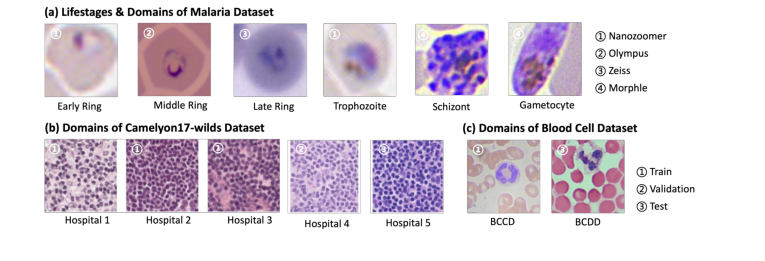Figure 2. Example images from our tested datasets

What the Evidence Proves

The experimental evidence, as summarized in Table 1, provides compelling proof that BeerLaNet's core mechanism—physics-informed, trainable stain disentanglement via algorithmic unrolling—works effectively in reality and offers superior cross-domain generalization compared to its baselines.

BeerLaNet achieved the best performance in both malaria parasite detection (mAP50 of 95.07% and mAP50-95 of 57.10%) and malaria parasite classification (Acc of 48.66% and RAcc of 90.33%). It also secured the second-highest performance in whole blood cell detection (mAP50 of 86.80% and mAP50-95 of 51.33%). While not always the absolute top performer on every single metric (e.g., Macenko achieved a slightly higher accuracy on C17test), the definitive evidence of BeerLaNet's superiority lies in its consistent and robust performance across all diverse tasks and datasets, as quantified by the Average Percent Underperformance (APU) metric.

BeerLaNet significantly outperformed all comparison methods in terms of APU, achieving 2.00 for detection tasks and 1.86 for classification tasks. This is a crucial piece of evidence. For instance, Macenko, while achieving the best accuracy on the Camelyon-17 WILDS C17test dataset (95.92%), suffered a substantial drop of over 10 percentage points on the C17val dataset (85.77%). Similar significant performance drops were observed for virtually all other baseline methods across different tasks or datasets. This inconsistency highlights their vulnerability to domain shifts.

The baselines, particularly those with generic designs or reliance on fixed templates, struggled to generalize when faced with larger color variations, such as those present in the malaria dataset (as visually suggested in Fig. 2). Their performance was often strong on datasets with relatively minor color shifts (like Camelyon17-WILDS or whole blood cells) but faltered dramatically under more challenging conditions. In contrast, BeerLaNet maintained a very competitive performance even when not the absolute best, demonstrating its ability to adapt to a wide range of staining and imaging conditions without prior knowledge or template selection. This consistent, high-level performance, ruthlessly exposed by the APU metric, is the undeniable evidence that BeerLaNet's physics-informed, end-to-end trainable approach effectively disentangles stain-invariant structural information, leading to robust cross-domain generalization in medical histology.

Limitations & Future Directions

While BeerLaNet demonstrates remarkable robustness and consistent performance across diverse medical histology tasks, it's important to acknowledge its inherent limitations and consider avenues for future development.

One subtle limitation, as noted by the authors, is that BeerLaNet is not always the absolute top-performing method for every single specific dataset or metric. For example, Macenko achieved a slightly higher accuracy on the Camelyon-17 WILDS C17test dataset. While BeerLaNet's strength lies in its consistent high performance across the board (evidenced by its superior APU), this suggests there might still be room for specialized optimization that could push its performance even higher on particular, less challenging domain shifts. The paper also doesn't explicitly detail the computational overhead of the unrolled network architecture compared to simpler baselines, which could be a practical consideration for extremely large whole slide images or real-time applications.

Looking forward, the authors propose exploring BeerLaNet's application to additional downstream tasks such as segmentation and other histopathological domains. This is a natural extension, given its plug-and-play design.

Beyond these, several discussion topics emerge for further developing and evolving these findings:

• Generalizability to Novel Stains and Imaging Modalities: The paper emphasizes BeerLaNet's ability to handle "arbitrary staining protocols." How well would it perform on entirely novel stains or imaging modalities (e.g., fluorescence microscopy, mass spectrometry imaging) that differ significantly from the H&E or Giemsa stains primarily used in the experiments? Future work could involve rigorous testing on a broader spectrum of unseen staining types to truly validate its "adaptive" claim.
• Interpretability and Clinical Utility of Disentangled Components: BeerLaNet extracts stain-invariant structural information (the D matrix). Can this disentangled representation be directly interpreted by pathologists or used for quantitative analysis beyond improving downstream task performance? Developing tools to visualize and quantify these components could provide new diagnostic insights and enhance trust in AI-driven pathology.
• Dynamic Hyperparameter Adaptation: The number of colored components ($r$) and unrolled iterations ($K$) are set as fixed hyperparameters. Could these be dynamically adapted based on the input image characteristics or the complexity of the staining protocol? An adaptive mechanism could further optimize performance and reduce the need for manual tuning.
• Integration with Multi-Modal Data: Histopathology often involves integrating information from various sources (e.g., molecular data, patient history). How could BeerLaNet's stain normalization be combined with multi-modal learning frameworks to provide a more comprehensive diagnostic picture?
• Robustness to Image Quality Degradations: While stain variability is addressed, real-world pathology images can suffer from other degradations like out-of-focus regions, dust, or compression artifacts (partially addressed for malaria classification). Can the physics-informed unrolling framework be extended to jointly normalize stains and correct for other common image quality issues?
• Ethical Considerations and Artifact Prevention: In medical diagnosis, introducing synthetic artifacts or "hallucinating" cellular structures is a critical concern, as noted for some GAN-based methods. While BeerLaNet aims to avoid this, continuous validation and perhaps even formal certification processes are needed to ensure that the normalization process never inadvertently obscures or alters diagnostically relevant features, even if overall accuracy improves.
• Computational Efficiency for Whole Slide Imaging: Processing gigapixel whole slide images (WSIs) is computationally demanding. While BeerLaNet is end-to-end trainable, its unrolled NMF mechanism might still be resource-intensive. Future research could focus on optimizing its computational efficiency, perhaps through more lightweight unrolling architectures or efficient hardware implementations, to enable real-time WSI analysis.

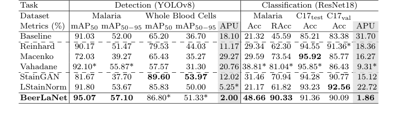Table 1. Comparison of Stain Normalization Techniques. The best and the second-best results are boldfaced or starred (*), respectively. (C17 denotes Camelyon17-WILDS)

Connections to Other Fields

Mathematical Skeleton

The pure mathematical core of this work is a structured Nonnegative Matrix Factorization (NMF) problem with combined $l_1$ and $l_2$ norm regularizations, which is solved using an unrolled alternating proximal gradient descent algorithm. This framework aims to decompose an input matrix into two non-negative factor matrices, promoting sparsity and low-rank propertys in the factors.

Adjacent Research Areas

Nonnegative Matrix Factorization (NMF)

The BeerLaNet model's foundation lies in Nonnegative Matrix Factorization, a widely used technique for dimensionality reduction and feature extraction in various fields. Specifically, the objective function in Eq. 4, which seeks to minimize $||x_0\mathbf{1}^T - X - SD^T||_F^2$ subject to $S, D \ge 0$ and additional regularizations, is a direct variant of the NMF problem. Here, the log-transformed image data is decomposed into a stain color matrix $S$ and an optical density matrix $D$. This mathematical structure, where a matrix is approximated by the product of two non-negative matrices, is central to applications like topic modeling in text analysis, spectral unmixing in hyperspectral imaging, and source separation in audio processing. For instance, in spectral unmixing, NMF is used to decompose a mixed pixel spectrum into a set of pure material spectra (endmembers) and their corresponding abundances, which is highly analogous to separating stain colors and their densities in histology images. A foundational work in NMF is by Lee and Seung (1999, Nature), a truly seminal paper.

Algorithmic Unrolling / Deep Unfolding

The method employs algorithmic unrolling, also known as deep unfolding, to transform the iterative optimization process for the structured NMF problem into a trainable deep neural network architecture. The alternating proximal gradient descent steps outlined in Algorithm 1, which update $x_0$, $D$, and $S$ by taking gradient steps and applying proximal operators for regularization and non-negativity constraints, are directly unrolled into a fixed number of network layers. This approach allows for end-to-end training of parameters like regularization strengths ($\gamma, \lambda$) and initializations ($S_{init}$) via backpropagation, leveraging the benefits of deep learning while maintaining the interpretability and theoretical guarantees of the underlying optimization algorithm. This technique has seen success in various signal processing and inverse problems, such as sparse coding, compressed sensing reconstruction, and image restoration, where iterative algorithms are converted into efficient, learnable deep models (e.g., Gregor & LeCun, 2010, ICML), a very clever idea.

---