CENet: Context Enhancement Network for Medical Image Segmentation
CENet boosts medical image segmentation by enhancing boundaries and preserving details across diverse image types.
Background & Academic Lineage
Historically, the precise delineation of anatomical structures, organs, and lesions in medical images was a purely manual task. Radiologists had to painstakingly draw boundaries pixel by pixel—a process that was incredibly time-consuming and expensive, effectively costing hundreds of dollars (e.g., \$150 per scan in labor) and driving the urgent need for automated systems. This problem birthed the field of automated medical image segmentation. The field was revolutonized by Fully Convolutional Networks (FCNs) and specifically the U-Net architecure, which introduced an encoder-decoder structure. The encoder compresses the image to understand "what" is in the scan, while the decoder expands it to pinpoint "where" it is. However, as medical imaging advanced, a critical challenge emerged: how do you teach a machine to simultaneously understand the broad, global context of an entire organ system while perfectly preserving the microscopic, fine-grained boundary details of a tiny tumor?
The fundamental limitation of previous approaches is a constant tug-of-war between capturing the big picture and retaining fine details. Traditional Convolutional Neural Networks (CNNs) have a limited "field of view," meaning they struggle to understand global relationships across large images. To fix this, researchers introduced Vision Transformers (ViTs), which look at the entire image at once. However, ViTs are computationally massive and notoriously bad at capturing local edge details. When previous models—even hybrid ones—attempted to pass fine-grained boundary details through the network to solve this, they suffered from a severe pain point: "over-enhancement." Without proper control mechanisms, amplifying edge details also amplifies background noise, leading to decoder-stage degradation. Existing models simply comprimise boundary details during the downsampling process, making highly accurate, multi-scale segmentation of complex organs nearly impossible. This forced the authors to create CENet to intelligently enhance boundaries without drowning the network in noise.
Here are a few highly specialized domain terms from the paper, translated into intuitive concepts:
- Skip Connections: In neural networks, these are architectural shortcuts that bypass certain layers to feed raw, detailed information directly to later stages of the model.
- Everyday Analogy: Imagine translating a highly detailed 1,000-page novel into a 10-page summary, and then asking an author to rewrite the full novel using only that summary. They would lose all the rich details. A skip connection is like handing the author the original character sketches and setting descriptions while they rewrite, ensuring the fine details aren't lost in translation.
- Receptive Field: The specific, restricted region of an input image that a particular part of the neural network is "looking at" at any given moment.
- Everyday Analogy: Think of looking at a massive, intricate mural through a cardboard paper towel tube. The small circle of the mural you can see at one time is your receptive field. To understand the whole story of the mural, you need a much wider tube.
- Downsampling: The process of intentionally reducing the spatial resolution of an image to compress information and extract high-level, semantic meaning.
- Everyday Analogy: It is like zooming out on a digital map on your phone. As you zoom out, you lose the names of individual streets and coffee shops (fine details), but you finally get to see the shape of the entire state or country (global context).
- Self-Attention Mechanism: A mathematical method that allows a model to weigh the importance of different parts of the input data relative to each other, deciding what to focus on.
- Everyday Analogy: Imagine you are at a loud, crowded cocktail party. Your brain naturally tunes out the background music and the clinking glasses to focus entirely on the voice of the person you are talking to. Self-attention does exactly this for data, deciding which pixels are the most important to "listen" to.
Key Mathematical Notation
| Notation | Description |
|---|---|
| $F$ | The input feature map processed by the network. |
| $\mathcal{D}(F, s)$ | Multi-scale downsampling operation applied to the feature map at scale $s$. |
| $\mathcal{U}(F, s)$ | Upsampling operation applied to the feature map at scale $s$. |
| $s_1, s_2, s_0$ | Specific scale parameters used for resizing feature maps (e.g., $0.75, 0.5, 1.0$). |
| $F_{u1}, F_{u2}$ | The resulting upsampled feature maps at different scales. |
| $F_{\text{edge}}$ | The isolated, refined edge details, mathematically defined as $\|F_{u1} - F_{u2}\|$. |
| $\lambda$ | A learnable weighting parameter vector ($\lambda \in \mathbb{R}^d$) used to scale the edge features. |
| $\tilde{F}$ | The final enhanced feature map after adding the weighted edge details back to the original input. |
| $\mathbf{g}$ | A global descriptor vector generated by pooling operations to capture channel-wise statistics. |
| $\mathbf{s}$ | The channel weights generated by the Channel Calibration Unit (CCU) to adaptively reweight features. |
| $F'$ | The reweighted output feature map after applying channel attention ($F \odot \mathbf{s}$). |
| $F'_i$ | Split portions of the feature map used in the Multi-scale Contextual Aggregator (MCA). |
| $f_{dk}$ | A depth-wise convolution operator with a specific kernel size and dilation rate $d_k$. |
| $\mathcal{C}_{\text{avg}}, \mathcal{C}_{\text{max}}, \mathcal{C}_{\text{std}}$ | Channel-wise average pooling, max pooling, and standard deviation pooling operations. |
| $G$ | A spatial descriptor created by combining different pooling operations in the Spatial Calibration Module. |
| $S$ | The combined output used to recalibrate the feature map via element-wise multiplication. |
Problem Definition & Constraints
Imagine trying to trace the exact outline of a complex, shape-shifting island on a highly pixelated satellite map. In the realm of medical image analysis, the starting point (Input) is a raw medical dataset—such as a CT scan, an MRI, or a dermoscopic photograph of a skin lesion. The desired endpoint (Output) is a precise, pixel-wise delineaton of anatomical structures, organs, or pathological lesions. The mathematical gap this paper attempts to bridge is the severe information loss that occurs when an image is compressed to understand its overall context, which inherently destroys the fine-grained spatial coordinates needed to draw accurate boundaries. The authors need a way to mathematically isolate and inject these missing edge details—which they calculate as the absolute difference between multi-scale upsampled features, $F_{edge} = |F_{u1} - F_{u2}|$—without drowning the system in irrelevant data.
In deep learning, fixing one problem almost always breaks another, and previous researchers have been trapped in a frustrating dilemma. If you use Convolutional Neural Networks (CNNs), the model becomes excellent at understanding local textures but fails to grasp the global context because of the limited receptive field of convolutional kernels. To fix this, researchers turned to Vision Transformers (ViTs), which use self-attention to look at the entire image at once. However, ViTs introduce a painful trade-off: while they capture global context beautifully, they severely underperform at modeling local edge representations. Furthermore, if you try to manually force the network to pay attention to fine-grained boundary features to fix this, you trigger a new problem: the lack of proper control mechanisms amplifies background noise, leading to "over-enhanced" representations that actually degrade the network's performance during the decoding stage. You are forced to choose between blurry boundaries, a lack of global understanding, or a noisy, unstable architecutre.
The authors hit several harsh, realistic walls that make this specific problem insanely difficult to solve:
- Quadratic Computational Complexity: While Transformers are powerful, their self-attention mechanisms scale quadratically with the input size, often expressed as $O(N^2)$. This creates a massive computational bottleneck and hits strict hardware memory limits, making them highly inefficient for large-scale, high-resolution medical applications.
- Destructive Downsampling: The hierarchical structure of modern neural networks relies heavily on downsampling to extract features. This physical constraint inherently comprimises boundary details and fine-grained semantic representations, which are mathematically difficult to recover once lost.
- Extreme Morphological Variability: Medical structures are not rigid. Organs and lesions are highly deformable, presenting diverse shapes, appearances, and pathological conditions across different patients. A fixed receptive field simply cannot adapt to this multi-scale variability.
- Noise Accumulation in Skip Connections: To recover lost details, networks use "skip connections" to bypass compression. However, without a way to filter this data, irrelevant background noise is passed directly into the decoder. The authors note that this creates a severe constraint where overly enhanced representations accumulate noise, requiring complex mathematical interventions to adaptively denoise the features without erasing the critical boundary details.
Why This Approach
When analyzing the landscape of medical image segmentation, the authors of CENet hit a very specific, frustrating wall. They realized that the traditional state-of-the-art (SOTA) architectures were fundamentally flawed for the harsh realities of clinical scans. Convolutional Neural Networks (CNNs) like U-Net are inherintly limited by the local receptive fields of their kernels—they simply cannot grasp the global context of a large, deformable organ. On the flip side, Vision Transformers (ViTs) emerged as the new gold standard for capturing global context via self-attention. However, the authors identified the exact moment ViTs failed: they severely underperform in modeling local fine-grained details (like the precise boundary of a lesion) and carry a crippling quadratic computational compexity that makes them highly inefficient for large-scale, high-resolution medical applications.
Even when previous researchers tried to mash these together into hybrid CNN-Transformer models, a new problem emerged. Forcing fine-grained edge features into the decoder without strict control mechanisms just flooded the network with noise, leading to decoder-stage degradation. The authors realized that a brute-force approach wasn't viable; they needed a highly controlled, mathematically rigorous filtering system. This is why the Context Enhancement Network (CENet) was the only viable solution.
To solve this, they engineered a "marriage" between the harsh constraints of medical imaging—where boundaries are fuzzy and organs vary wildly in size—and a unique dual-filtering architecture. They introduced the Dual Selective Enhancement Block (DSEB) into the skip connections. Instead of blindly passing features from the encoder to the decoder, the DSEB actively isolates and amplifies edge details using a Feature Edge Amplifier (FEA). It does this by calculating the difference between features at different scales:
$$F_{edge} = |F_{u1} - F_{u2}|$$
where $F_{u1}$ and $F_{u2}$ are upsampled features from different downsampling scales. This isolated edge map is then injected back into the original feature map:
$$\tilde{F} = F + \lambda F_{edge}$$
where $\lambda \in \mathbb{R}^d$ acts as a weighting parameter.
But here is where the comparative superiority truly shines. If you amplify edges, you usually amplify high-dimensional noise. To combat this, the authors integrated Differential Attention (DiffAtt). By calculating separate attention maps and subtracting them, they effectively cancel out redundant attention and imbalanced token importance. It acts as an active noise-canceling headphone for the neural network.
Furthermore, the decoder utilizes the Context Feature Attention Module (CFAM) to prevent the network from choking on overly enhanced representations. It uses a Channel Calibration Unit (CCU) to compress and adaptively reweight the channels using a global descriptor $\mathbf{g}$:
$$\mathbf{g} = [\mathcal{P}_{avg}(F); \mathcal{P}_{max}(F); \mathcal{P}_{std}(F)]$$
This is followed by a Multi-scale Contextual Aggregator (MCA) that splits the features and processes them through parallel dilated depth-wise convolutions. This structural advantage allows the network to look at multiple scales simultaneously without the massive parameter bloat of traditional dense layers.
To be honest, the paper doesn't explicitly provide the exact Big-O mathematical notation for how much memory complexity is reduced compared to standard ViTs, but they explicitly reject standard Transformers due to their quadratic inefficiency. By utilizing depth-wise convolutions and channel reduction, CENet achieves a qualitatively superior, lightweight represntation that easily outperforms heavier models.
Finally, the paper explains exactly why other popular approaches fail. While they don't explicitly mention rejecting GANs or Diffusion models—to be completely transparent, those generative models likely struggle with the deterministic precision required here anyway—they heavily critique existing localized self-attention and hybrid models. Those alternatives focus too much on "body features" rather than "edge information" and lack the adaptive denoising required to handle the noise accumulation. CENet's inclusion of the weighted Non-local Block (wNLB) at the end of the CFAM perfectly models long-range spatial dependencies to suppress over-attended, irrelevant details (like hairs in dermoscopy images), proving that controlled, context-aware enhancement is overwhelmingly superior to the previous gold standard.
Mathematical & Logical Mechanism
To understand the brilliance of the Context Enhancement Network (CENet), we first need to understand the fundemental tug-of-war in medical image segmentation. Imagine trying to trace the exact outline of a tumor or an organ (like a kidney) from a blurry, grayscale medical scan. If you zoom in too much, you see the precise edges but lose track of where you are in the body (loss of global context). If you zoom out, you know exactly where you are, but the fine boundaries blur into pixels (loss of local detail).
Historically, Convolutional Neural Networks (CNNs) were the "zoomed-in" experts, looking through a tiny sliding window, while Vision Transformers (ViTs) were the "zoomed-out" experts, looking at the whole image but struggling with fine, localized boundaries. Furthermore, when engineers tried to combine them, the networks often suffered from "over-enhancement"—amplifying background noise alongside the actual organs, leading to degraded predictions.
The authors of CENet solved this by designing a highly controlled, multi-scale architecure that acts like a smart magnifying glass. It selectively enhances boundaries while using a sophisticated gating mechanism to suppress irrelevant noise.
Here is the mathematical autopsy of how they achieved this.
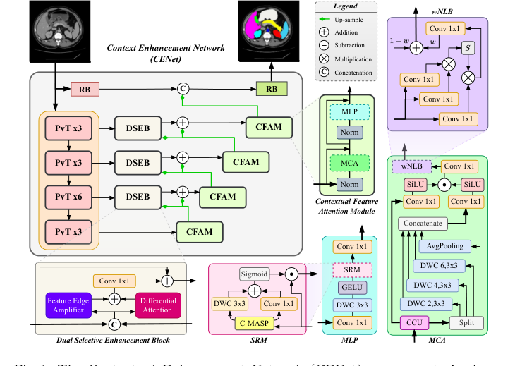 Figure 1. The Contextual Enhancement Network (CENet) uses a pretrained en- coder to generate multi-resolution features, processed by the DSEB as skip con- nections. The decoder refines these features via the CFAM, which includes a CCU, MCA, wNLB, and MLP
The Master Equations
The beating heart of CENet relies on two interconnected mathematical engines. The first is the Dual Selective Enhancement Block (DSEB), which rescues boundary details. The second is the Multi-scale Contextual Aggregator (MCA), which intelligently fuses different zoom levels without overwhelming the network with noise.
The boundary enhancement engine:
$$ \tilde{F} = F + \lambda F_{edge} $$
The multi-scale context gating engine:
$$ F_{MCA} = \Big( \text{SiLU}(f_{1\times1}(F_{cat})) \odot \text{SiLU}(f_{1\times1}(F')) \Big) + F $$
Tearing the Equations Apart
Let's dissect every single gear and spring in these mechanims.
From the Boundary Engine:
* $F$: The original input feature map. Physically, this is the baseline reality of the image at a specific layer—the raw, unedited signal.
* $F_{edge}$: The isolated edge details. The authors compute this by downsampling and upsampling the image at different scales and taking the absolute difference ($|F_{u1} - F_{u2}|$). Logically, this acts as a high-pass filter, capturing only the sharp transitions (the boundaries of organs).
* $\lambda$: A learnable weighting parameter (a vector in $\mathbb{R}^d$). This acts as a volume dial for the edges, allowing the network to decide how much boundary enhancement is actually needed for each specific channel.
* $+$ (Addition): Why add instead of multiply? Addition acts as an overlay. We are taking the baseline image ($F$) and drawing the enhanced boundaries ($\lambda F_{edge}$) on top of it. If we used multiplication, any region without an edge (where $F_{edge} \approx 0$) would wipe out the entire image, turning the inside of the organs pitch black!
From the Context Gating Engine:
* $F_{cat}$: The concatenated multi-scale features. The network splits the image and looks at it through different "dilated" lenses (looking at neighbors 3, 5, and 8 pixels away), then stacks them together. This represents the "global context" or the forest.
* $F'$: The channel-calibrated feature map. This is the original signal that has been reweighted so that the most important feature channels are prioritized. This represents the "local detail" or the trees.
* $f_{1\times1}$: A point-wise convolution. Mathematically, it is a linear transformation across the depth of the feature map. Logically, it acts as a bartender, mixing the different channels of information together without changing the spatial width or height of the image.
* $\text{SiLU}$: The Sigmoid Linear Unit activation function. It allows strong positive signals to pass through linearly but smoothly squashes negative signals toward zero. It acts as a soft, continuous gatekeeper.
* $\odot$ (Hadamard Product): Element-wise multiplication. This is the most critical operator. Why multiplication instead of addition? Multiplication acts as a logical AND gate (a filter). The left side of the equation evaluates the context ($F_{cat}$), and the right side evaluates the local features ($F'$). By multiplying them, the network only allows a signal to pass if both the local details and the global context agree that it is important. It actively mutes irrelevant background noise.
* $+$ (Residual Addition): After the complex gating mechanism decides what to enhance, it is added back to the original input $F$. This is a residual connection. It ensures that the network never forgets the original image, acting as a safety net against over-processing.
Step-by-Step Flow
Let’s trace the exact lifecycle of a single abstract data point—say, a high-dimensional vector representing a tiny pixel on the boundary of a stomach.
- Baseline Entry: The stomach boundary pixel enters the DSEB block as part of the feature map $F$.
- Edge Extraction: The network shrinks and expands the image around this pixel. Because it's on a boundary, the pixel shifts slightly during this process. The network subtracts the two versions, isolating the sharp transition. Our pixel is now glowing in the $F_{edge}$ map.
- Boundary Injection: The network scales this glow by $\lambda$ and adds it back to the original pixel ($+$). The stomach boundary is now crisp and well-defined ($\tilde{F}$).
- Context Gathering: The pixel moves into the CFAM decoder. It is split into clones. One clone looks at its immediate neighbors; another looks 8 pixels away to realize, "Ah, I am next to the liver." These perspectives are stacked together into $F_{cat}$.
- The Gating Interrogation: The context ($F_{cat}$) and the pixel's own calibrated identity ($F'$) are both mixed by $f_{1\times1}$ and smoothed by $\text{SiLU}$. They meet at the multiplication operator ($\odot$). The context says, "This is a valid organ boundary," outputting a high value (e.g., 0.9). The local feature says, "I am a sharp edge," outputting a high value (e.g., 0.8). They multiply ($0.9 \times 0.8 = 0.72$), surviving the filter. (If this pixel were just a random hair on the skin, the context would output 0.01, and the multiplication would instantly kill the noise).
- Final Recombination: This refined, context-approved signal is added ($+$) back to the raw pixel $F$. The data point exits the module, perfectly enhanced and ready for the final segmentation map.
Optimization Dynamics
How does this mechanical assembly line actually learn to segment organs?
The learning process is driven by the gradients flowing backward from the loss function (specifically, the BDoU Loss, which penalizes the network heavily if it gets the boundaries wrong).
The architecture shapes a highly favorable loss landscape. Because of the heavy use of residual additions ($+$), the gradients have a "fast-pass" highway to flow directly from the end of the network all the way back to the early layers without vanishing.
Meanwhile, the gating mechanism ($\odot$) acts as a dynamic gradient router. During backpropagation, if the SiLU gate for a specific region was closed (near zero) during the forward pass because it was deemed irrelevant noise, the gradient flowing back through that path is also multiplied by zero. This effectively freezes learning for dead weight and forces the optimizer to concentrate all its updating power on the weights responsible for the salient regions (the organs and boundaries).
Finally, to prevent the network from getting too excited and creating runaway feedback loops (where enhanced features keep getting enhanced until they explode into noise), the authors placed a weighted Non-Local Block (wNLB) at the end of the module. This acts as a spatial regularizer. It looks at the entire image at once and smooths out any isolated spikes of over-enhancement, ensuring the optimization trajectory remains stable, smooth, and converges to a highly accurate, boundary-perfect segmentation.
Results, Limitations & Conclusion
To truly appreciate the Context Enhancement Network (CENet), we first need to understand the fundamental problem of medical image segementation. Imagine you are tasked with tracing the exact borders of a country on a highly detailed, yet slightly blurry, satellite map. In the medical field, this "tracing" is pixel-wise segmentation—identifying the exact boundaries of organs, tumors, or lesions from raw CT, MRI, or skin scans.
Historically, scientists used Convolutional Neural Networks (CNNs) for this. CNNs act like a magnifying glass; they are excellent at looking at local textures but terrible at understanding the global context (the "big picture"). Recently, Vision Transformers (ViTs) entered the scene. ViTs act like a satellite view; they understand the global context perfectly but often blur out the fine, local boundary details. When engineers try to combine these two approaches, or when they shrink the images to save computational power (downsampling), the delicate borders of organs are compromised.
The core motivation of this paper is to solve a frustrating paradox: if you try to mathematically force a network to pay more attention to fine edges, you inevitably amplify the background noise (like static on a TV or hairs on a skin scan). The authors needed to build a system that could enhance the borders of complex, deformable organs without causing "over-enhancement" or degrading the network's learning process.
The Mathematical Core: What Problem Was Solved and How?
The authors architected CENet to intercept and refine the flow of visual information using two brilliant mathematical interventions: the Dual Selective Enhancement Block (DSEB) and the Contextual Feature Attention Module (CFAM).
1. Isolating the Edges (DSEB)
Instead of just guessing where the edges are, the DSEB mathematically isolates them using a Feature Edge Amplifier (FEA). The network takes an input feature map $F$ and scales it down and back up at different ratios ($s_1 = 0.75$ and $s_2 = 0.5$).
$$F_{u1} = U(\mathcal{D}(F, s_1), s_0), \quad F_{u2} = U(\mathcal{D}(F, s_2), s_0)$$
Here, $\mathcal{D}$ is downsampling and $U$ is upsampling. Because these two versions of the image were compressed differently, subtracting them cancels out the broad, flat areas (like the middle of an organ) and leaves only the sharp, high-frequency edge details:
$$F_{edge} = |F_{u1} - F_{u2}|$$
This pure "edge map" is then weighted by a learned parameter $\lambda$ and added back to the original feature map:
$$\tilde{F} = F + \lambda F_{edge}$$
2. Taming the Noise (CFAM)
Once the edges are enhanced, the network risks becoming overwhelmed by noise. The CFAM acts as a multi-stage filtration system to prevent these overly enhanced represntations from ruining the final output.
First, it uses a Channel Calibration Unit (CCU) to figure out which "channels" (layers of visual data) are actually important. It does this by pooling the data in three different ways—average, maximum, and standard deviation—to create a global descriptor $\mathbf{g}$:
$$\mathbf{g} = [\mathcal{P}_{avg}(F); \mathcal{P}_{max}(F); \mathcal{P}_{std}(F)]$$
This descriptor generates a set of weights $\mathbf{s}$ that scales the original features: $F' = F \odot \mathbf{s}$.
Later in the CFAM, a Spatial Calibration Module (SRM) performs a similar trick for spatial locations, using parallel convolutions to capture both pixel-wise and neighborhood interactions:
$$S = \sigma(f_{1\times1}(G) + f_k^{dw}(G))$$
$$F_{recal} = F_{MCA} \odot S$$
By combining the edge-boosting of DSEB with the ruthless noise-filtering of CFAM, the authors solved the paradox: they achieved hyper-sharp boundaries without the static.
The Experimental Architecure: Proving the Claims
The authors did not just throw their model at a dataset and boast about a 1% accuracy bump. They designed a highly hostile proving ground to ruthlessly validate their mathematical claims.
The Victims (Baselines):
They pitted CENet against a massive roster of state-of-the-art models. The victims included pure CNNs (U-Net, DeepLabv3+), pure Transformers (Swin-Unet, MissFormer), and heavy-hitting hybrid models (TransUNet, MSA$^2$Net, UCTransNet).
The Definitive Evidence:
To prove their model wasn't just memorizing one specific type of image, they tested it across entirely different medical domains: internal radiology (3D CT and MRI scans of kidneys, stomachs, and hearts) and external dermoscopy (2D photos of skin lesions). CENet defeated the baselines across the board, achieving a massive 92.18% DICE score on the ACDC cardiac dataset.
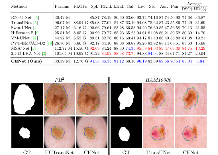 Figure 3. Qualitative comparison of CENet and previous methods across skin benchmarks
But the undeniable, smoking-gun evidence wasn't the metrics—it was the visual feature heatmaps and the ablation study. The authors literally opened up the "brain" of the network to show where it was looking.
1. Before DSEB: The network's attention was diffuse and scattered.
2. After DSEB: The attention snapped tightly to the borders of the organs.
3. After wNLB (the denoising mechanism): The network actively suppressed irrelevant details. In the skin lesion dataset, you can visually see the network ignoring physical hairs on the patient's skin to focus purely on the lesion boundary.
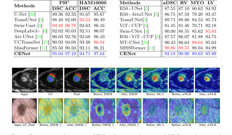 Figure 4. Feature visualization in CENet: first row shows an ACDC sample, second row a PH2 example
Furthermore, they systematically dismantled their own model (turning off DSEB, FEA, and CFAM one by one). The ablation study proved that without the specific mathematical combination of edge-amplification and noise-suppression, the model's performance collapsed.
Future Discussion Topics
Based on the brilliant mechanics introduced in this paper, here are several avenues for future exploration and critical debate:
- The Cost of Multi-Scale Processing vs. Clinical Reality:
CENet relies heavily on multi-scale downsampling, upsampling, and dilated convolutions. While highly accurate, how does this impact inference time? If a hospital wants to deploy this on a standard \$150 clinical GPU rather than an NVIDIA A100, will the complex gating mechanisms of the CFAM become a bottleneck? We must discuss how to distill these heavy mathematical operations into lighter, real-time architectures for emergency room diagnostics. - The "Fuzzy Boundary" Dilemma:
The DSEB module assumes that a sharp boundary is always the ground truth. However, in oncology, certain aggressive, infiltrating tumors (like Glioblastoma in the brain) inherently lack sharp boundaries; they fade into healthy tissue. How might the absolute difference mechanism ($|F_{u1} - F_{u2}|$) behave when the biological ground truth is a gradient rather than an edge? Could this mathematical strictness accidentally force the network to hallucinate a hard border where none exists? - Evolution to Continuous 3D Spatial Dependencies:
The current model processes 3D MRI and CT scans as a series of 2D slices. While the wNLB (weighted Non-local Block) captures long-range spatial dependencies within a slice, it ignores the Z-axis (depth). How can we mathematically evolve the Channel Calibration Unit (CCU) and Spatial Calibration Module (SRM) to process true volumetric tensors without causing an exponential explosion in computational complexity?
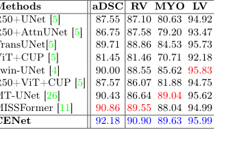 Table 2. Evaluation results on the skin benchmarks (PH2 and HAM10000) and ACDC dataset
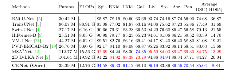 Table 1. Evaluation results on the Synapse dataset (blue indicates the best and red the second best results)