Cross-Modal Brain Graph Transformer via Function-Structure Connectivity Network for Brain Disease Diagnosis
Multi-modal brain networks represent the complex connectivity between different brain regions from both functional and structural perspectives, which is of great significance for brain disease diagnosis.
Background & Academic Lineage
To understand where this problem comes from, we have to look at how neuroscientists and computer scientists have historically tried to diagnose complex brain diseases like Alzheimer's Disease (AD) or Autism Spectrum Disorder (ASD). In the early days of neuroimaging, reasearchers relied on single types of brain scans to look for anomalies. Eventually, the field realized that the brain operates as a highly complex, interconnected network. This led to the use of two distinct perspectives: functional connectivity (how different brain regions activate together, measured by fMRI) and structural connectivity (the actual physical nerve fibers connecting them, measured by DTI). The specific problem of fusing these two modalities emerged because brain diseases often disrupt both the physical wiring and the communication patterns simultaneously. Diagnosing them accurately requires understanding the deeply coupled relationship between structure and function, rather than looking at either in isolation.
What was the fundamental limitation that forced the authors to write this paper? Previous approaches hit a major wall when trying to combine these two types of data. Graph Neural Networks (GNNs) were popular, but they only passed information locally between neighboring nodes, completely missing the widespread, long-range dependencies in the brain. To fix this, some recent models introduced Transformers, which are excellent at seeing the big picture. However, existing multi-modal models simply treated functional and structural data as two separate, parallel views and merely fused their final features together at the end. They completely neglected the supporting role of structural connectivity—specifically, how the physical wiring should dictate or guide the functional comunication. The authors realized that without using the physical structure to explicitly guide the model's "attention" to functional data, previous models were leaving critical diagnostic information on the table.
Here are a few highly specialized terms from the paper, translated into everyday concepts:
- Functional Connectivity Network (fMRI): Think of this as the real-time phone call traffic between different cities. It doesn't show the phone lines themselves, but it reveals which cities are frequently talking to each other at the exact same time.
- Structural Connectivity Network (DTI): This is the physical infrastructure—the actual fiber-optic cables or concrete highways built between those cities. Even if two cities aren't talking right now, the physical highway exists.
- Region of Interest (ROI): Imagine looking at a map of a country; an ROI is simply a specific city or state. In the brain, it's a specific anatomical area (like the hippocampus) that researchers monitor for activity or connections.
- Cross-modal TopK Pooling: Imagine a government committee trying to downsize a massive national map to only the top $k$ most critical cities to monitor for a crisis. Instead of just looking at population size (one modality), they evaluate both the physical highway infrastructure and the phone traffic (cross-modal) to select the most important cities, discarding the rest to simplify their analysis.
Let's organize the key mathematical notations used to solve this problem.
| Notation | Type | Description |
|---|---|---|
| $\mathbf{X}_{s}$ | Variable | The structural connectivity matrix obtained from DTI images. |
| $\mathbf{X}_{s,(i,j)}$ | Variable | The number of physical fiber connections between ROI $i$ and ROI $j$. |
| $\mathbf{M}^0$ | Parameter | The initial enhanced mask, reconstructed from filtered strutural features to guide the Transformer. |
| $\mathbf{X}_f^{l-1}$ | Variable | The input node feature matrix (representing functional connectivity) at the $l$-th layer. |
| $\mathbf{M}^{l-1}$ | Variable | The enhanced mask at the $l$-th layer, used to guide the attention mechanism based on physical wiring. |
| $\mathbf{W}_Q^{l,z}, \mathbf{W}_K^{l,z}, \mathbf{W}_V^{l,z}$ | Parameter | Learnable weight matrices for Query, Key, and Value in the multi-head self-attention mechanism. |
| $\mathbf{S}^l$ | Variable | The final score vector that reflects the cross-modal importance of each node for pooling. |
| $\mathbf{i}$ | Variable | The index vector storing the top $k$ selected nodes after the pooling process. |
Problem Definition & Constraints
To understand the exact problem this paper tackles, we first need to define where we are starting and where we want to go.
The Starting Point (Input): We begin with two distinct types of brain network data extracted from neuroimaging.
1. Functional Connectivity (FC): Derived from fMRI scans, this captures how different brain regions "fire" together. Mathematically, it is represented as an initial node feature matrix $\mathbf{X}^0_f \in \mathbb{R}^{N^0 \times N^0}$, obtained by calculating the Pearson correlation coefficient between $N^0$ different Regions of Interest (ROIs).
2. Structural Connectivity (SC): Derived from DTI scans, this represents the actual physical "wiring" or nerve fiber tracts connecting these regions, represented as a matrix $\mathbf{X}_s \in \mathbb{R}^{N^0 \times N^0}$.
The Goal State (Output): The ultimate objective is to output a highly accurate classification probability $P(c)$ to determine if a patient has a specific brain disease (like Alzheimer's Disease or Autism Spectrum Disorder) or is a normal control.
The Mathematical Gap: The missing link here is how to effectively mathematically weave the physical wiring (structure) into the functional firing (activity). Previous researchers simply extracted features from both networks independently and concatenated them at the end (fusion in the feature dimensons). They failed to capture the deep, coupled interdependence between the two. The authors of this paper realized that structural connectivity should act as a physical map to guide and enhance the mathematical attention paid to functional connectivity.
However, bridging this gap introduces a painful dilemma that has trapped previous researchers.
The Dilemma:
In brain network analysis, diagnosing a disease requires understanding how distant brain regions communicate. This means the model must capture "long-range dependencies."
Here is the trade-off: If you use Graph Neural Networks (GNNs), you successfully capture the local physical topology of the brain, but GNNs are notoriously bad at capturing long-range dependencies due to a phenomenon called over-smoothing. On the other hand, if you use a standard Transformer architecture, the self-attention mechanism is brilliant at capturing long-range dependencies. However, standard Transformers are "topology-blind"—they treat every brain region as equally connected, completely ignoring the actual physical nerve fiber highways of the brain.
If you try to force a Transformer to learn the brain's topology from scratch, you run into severe computational bloat and noise. You are stuck: use GNNs and lose the long-distance functional misfires, or use Transformers and lose the physical structural constraints.
The Harsh Walls and Constraints:
To solve this dilemma, the authors hit several harsh, realistic walls that make this problem insanely difficult:
- Extreme Data Skewness: You cannot just feed the raw structural connectivity matrix $\mathbf{X}_s$ into a neural network. The number of physical fiber connections between two brain regions, $\mathbf{X}_{s,(i,j)}$, has a wildly skewed distribution ranging from absolute zero to several thousands. To make this mathematically stable, the authors were forced to apply a strict logarithmic transformation $\mathbf{X}_{s,(i,j)} = \log_{10}(\mathbf{X}_{s,(i,j)} + 1)$ followed by standard normalization just to make the sample means conform to a normal distribution.
- The Curse of Dimensionality and Noise: The brain is parcellated into many ROIs (nodes). Computing dense attention across all ROIs across multiple modalities is computationally expensive and introduces massive noise, as not all brain regions are relevant to a specific disease. The graph size must be reduced.
- The Cross-Modal Pooling Constraint: Reducing the graph size requires dropping nodes (pooling). But how do you drop nodes without accidentally throwing away the exact biomarker needed for diagnosis? If you only look at functional data to drop nodes, you might discard a region with critical structural damage. The constraint here is that node importance must be evaluated from both functional and structural perspectives simultaneously before deciding to keep or discard it. To be honest, I'm not completly sure how previous unimodal pooling methods justified ignoring structural damage, but this paper overcomes it by projecting both the structural mask and functional features onto learnable vectors to calculate a unified cross-modal score $\mathbf{S}^l$ to represnt the final node importance.
Why This Approach
The Breaking Point of Traditional Methods
To understand why the authors chose this specific architecture, we have to look at the exact moment traditional methods hit a wall. In brain network analysis, the goal is to diagnose diseases like Alzheimer's or Autism by looking at how different regions of the brain (Nodes) communicate with each other.
For a long time, Graph Neural Networks (GNNs) were the gold standard for this. However, the authors realized a fundemental flaw: GNNs operate on a "local information propagation" mechanism. They only talk to their immediate neighbors. But the human brain is highly complex, and diseases often disrupt long-range dependencies—meaning a region in the front of the brain might miscommunicate with a region in the back. Just like you wouldn't spend USD 150 on a local city map when you need to navigate a cross-country highway system, GNNs were simply too myopic for whole-brain analysis.
Transformers, with their self-attention mechanisms, solve this by looking at the entire graph at once. But standard Transformers (like BrainNetTF) introduced a new problem: they only looked at functional MRI (fMRI) data, completely ignoring the physical neural fiber wiring (DTI data). Other multi-modal methods tried to fix this by processing functional and structral data side-by-side as "multi-view" data. The authors realized this was insufficient because it ignored the supporting role of physical wiring. You can't just mash the two datasets together; the physical wiring must explicitly guide the functional activity. This realization made the Cross-Modal Brain Graph Transformer (CBGT) the only viable solution.
The Structural Advantage and Benchmarking Logic
Beyond just hitting higher accuracy numbers on a chart, this method is qualitatively superior because of how it handles graph complexity and noise. Brain networks are incredibly noisy and high-dimensional. If you try to process every single connection at every layer, you drown in computational overhead and irrelevant data.
To solve this, the authors introduced a "Cross-Modal TopK Pooling" module. Instead of relyng on a massive, static graph, the model dynamically evaluates the importance of each brain region (ROI) by fusing both functional and structural scores:
$$ \mathbf{S}^l = \sigma(\mathbf{S}^l \cdot \mathbf{W}^l + \mathbf{b}^l) $$
Based on this score vector $\mathbf{S}^l$, the model selects only the top $k$ most critical nodes:
$$ \mathbf{i} = \text{topk}(\mathbf{S}^l, k) $$
While the paper doesn't explicitly frame this as a strict $O(N^2)$ to $O(N)$ memory reduction in Big-O notation, the structural advantage is exactly that: it drastically shrinks the graph size layer by layer. By filtering out non-essential brain regions, it preserves only the most critical biomarkers (like the precuneus or hippocampus), making the model overwhelmingly superior to previous methods that forced the network to memorize the entire noisy graph.
The Perfect Marriage of Problem and Solution
The harshest constraint in this problem was finding a way to mathematically force the Transformer to care about the physical brain wiring when it is looking at functional activity.
The authors achieved a brilliant "marriage" between this constraint and their solution through the creation of an Enhanced Mask, denoted as $\mathbf{M}^{l-1}$. First, they use XGBoost to filter out unimportant physical connections from the structural data, leaving only the most influential physical pathways. Then, they inject this structural mask directly into the heart of the Transformer's functional self-attention mechanism:
$$ \mathbf{T}^{l,z} = \text{softmax} \left( \frac{\mathbf{W}_Q^{l,z} \mathbf{X}_f^{l-1} \left( \mathbf{W}_K^{l,z} \mathbf{X}_f^{l-1} \right)^\top}{\sqrt{d_K^{l,z}}} \odot (1 + \mathbf{M}^{l-1}) \right) $$
Look closely at the right side of that equation: $\odot (1 + \mathbf{M}^{l-1})$. The left side of the element-wise multiplication ($\odot$) is the standard attention score showing how much two brain regions are functionally firing together. By multiplying it by $(1 + \mathbf{M}^{l-1})$, the model mathematically amplifies the attention score if and only if there is also a strong physical neural fiber connecting them. It is a perfectly elegant way to make structure dictate function.
The Road Not Taken
The paper explicitly explains why GNNs were rejected (inability to capture long-range dependencies) and why standard multi-modal fusion was rejected (treating structure and function as separate but equal, rather than interdependent).
To be honest, I'm not completely sure how generative models like GANs or Diffusion models would perform here, as the authors do not mention them at all. However, logically, GANs and Diffusion models are designed to generate new data distributions from noise. The problem defined here is strictly a discriminative graph classification task (e.g., diagnosing Alzheimer's vs. Normal Control). Using a Diffusion model to classify a graph would be computationally exorbitant and architecturally misaligned with the goal of identifying specific, localized brain biomarkers. Therefore, a discriminative Transformer with cross-modal pooling was the most direct and logical path to take.
Mathematical & Logical Mechanism
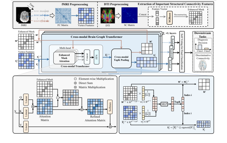 Figure 1. The proposed cross-modal brain graph Transformer framework
To understand the profound leap this paper makes, we first need to understand the human brain as a dual-layered network: a combination of "hardware" and "software."
In neuroimaging, the "hardware" is measured by Diffusion Tensor Imaging (DTI), which maps the actual, physical neural fibers connecting different brain regions. This is called structural connectivity. The "software" is measured by functional Magnetic Resonance Imaging (fMRI), which tracks blood flow to see which brain regions are firing at the same time. This is called functional connectivity.
For years, doctors and AI researchers trying to diagnose brain diseases (like Alzheimer's or Autism) faced a massive constraint: they either looked at the hardware, the software, or just clumsily mashed the two datasets together. Standard Graph Neural Networks (GNNs) are short-sighted—they only look at immediate neighboring brain regions. Transformers, on the other hand, are brilliant at seeing long-range dependencies (how a region in the front of the brain affects one in the back), but they easily get lost in the noise of the brain's massive functional data if they don't have a map.
The authors of this paper solved this by creating a Cross-Modal Brain Graph Transformer (CBGT). They mathematically force the AI to use the physical hardware (structural connectivity) as a guiding blueprint to better understand the software (functional connectivity).
Here is the absolute core mathematical engine that powers this cross-modal fusion.
$$ \mathbf{T}^{l,z} = \text{softmax} \left( \frac{\mathbf{W}_Q^{l,z} \mathbf{X}_f^{l-1} \left( \mathbf{W}_K^{l,z} \mathbf{X}_f^{l-1} \right)^\top}{\sqrt{d_K^{l,z}}} \odot \left( 1 + \mathbf{M}^{l-1} \right) \right) $$
$$ \mathbf{h}^{l,z} = \mathbf{T}^{l,z} \mathbf{W}_V^{l,z} \mathbf{X}_f^{l-1} $$
Let us tear these equations apart piece by piece to understand how they breathe life into the model.
- $\mathbf{X}_f^{l-1}$: This is the input node feature matrix at layer $l-1$. Physically, it represnts the "software" signals—the functional brain activity of different regions.
- $\mathbf{W}_Q^{l,z}, \mathbf{W}_K^{l,z}, \mathbf{W}_V^{l,z}$: These are learnable weight matrices for the Query, Key, and Value in attention head $z$. Logically, they act as translators. They use matrix multiplication to rotate and project the raw brain signals into a new mathematical space where regions can ask questions (Query), provide answers (Key), and offer substance (Value).
- $(\dots)^\top$: The transpose operator. It flips the Key matrix so that it can be multiplied against the Query matrix. This dot product measures the raw similarity or "alignment" between two brain regions' activities.
- $\sqrt{d_K^{l,z}}$: The square root of the dimension of the Key vectors. This acts as a thermodynamic thermostat. When you multiply large vectors, the resulting numbers can explode, pushing the softmax function into flat, dead zones where learning stops. Division is used here to shrink the variance and keep the mathematical engine running smoothly.
- $\mathbf{M}^{l-1}$: The enhanced mask derived from the structural connectivity network. This is the "hardware" map, pre-filtered by an XGBoost algorithm to only keep the most critical physical nerve connections.
- $1 + \mathbf{M}^{l-1}$: The structural bias. Why use addition here? The number $1$ acts as a baseline. If $\mathbf{M}$ is $0$ (meaning no physical wire connects two regions), the term simply becomes $1$. This ensures the baseline functional informtion isn't wiped out. If there is a physical connection, $\mathbf{M}$ adds to the $1$, amplifying the connection.
- $\odot$: The Hadamard product (element-wise multiplication). This acts as a magnifying glass. It scales the functional attention scores directly using the structural blueprint. Multiplication is used instead of addition here so that the structural mask acts as a proportional multiplier—scaling up the attention exactly where the physical architecure of the brain supports it.
- $\text{softmax}$: A normalization function. It acts as a strict budgeter, forcing all the raw, boosted similarity scores to sum up to exactly $1.0$ (or 100%). It converts raw math into a probability distribution.
- $\mathbf{T}^{l,z}$: The final attention matrix. This is the routing network, a master ledger telling every brain region exactly how much it should listen to every other region.
- $\mathbf{h}^{l,z}$: The output hidden state. This is the updated, enriched signal of the brain regions after they have communicated with each other.
To see this in action, let us trace the exact lifecycle of a single abstract data point—say, the signal from the Hippocampus—passing through this equation.
First, the raw functional signal of the Hippocampus ($\mathbf{X}_f$) enters the assembly line and is multiplied by $\mathbf{W}_Q$ to forge a Query vector. It is essentially shouting into the void: "Who is firing in sync with me?" Simultaneously, all other brain regions, like the Prefrontal Cortex, generate their Key vectors ($\mathbf{W}_K \mathbf{X}_f$). The Hippocampus's Query is multiplied against the Prefrontal Cortex's Key. If their functional signals match, the resulting score is high.
Next, this raw score is divided by $\sqrt{d_K}$ to cool it down and prevent mathematical overflow. Now comes the cross-modal magic. The system checks the structural mask $\mathbf{M}$. Is there an actual, physical neural fiber connecting the Hippocampus to the Prefrontal Cortex? If yes, the mask $\mathbf{M}$ holds a high value, and the element-wise multiplication $\odot (1 + \mathbf{M})$ massively boosts their connection score. If no physical wire exists, the score is multiplied by $1$, leaving it unchanged.
The softmax function then clips and squashes all these scores into percentages. Let's say the Hippocampus decides to pay 80% of its attention to the Prefrontal Cortex. Finally, the Hippocampus absorbs 80% of the Prefrontal Cortex's Value vector ($\mathbf{W}_V \mathbf{X}_f$), updating its own internal state to become $\mathbf{h}$. The Hippocampus has now successfully updated its software based on the constraints of the brain's hardware.
How does this mechanism actually learn and converge? The optimization dynamics here are beautifully constrained. The model is supervised at the very end by a Cross-Entropy loss function, which measures how wrong the model's final disease diagnosis is.
During backpropagation, the gradients flow backward from the final classification, through a TopK pooling layer (which dynamically learns to drop useless brain regions and keep only the most critical biomarkers), and into the Transformer layers. Because of the structural mask $\odot (1 + \mathbf{M})$, the loss landscape is fundamentally reshaped. In a standard Transformer, the loss landscape is chaotic because the model can easily overfit to random, noisy functional correlations (e.g., two brain regions firing together by pure coincidence).
However, the structural mask acts as a deep, smooth valley in the loss landscape. It acts as a physical prior, forcing the gradients to flow much more strongly along actual biological pathways. The Adam optimizer updates the weight matrices ($\mathbf{W}_Q, \mathbf{W}_K, \mathbf{W}_V$) iteratively, but it is constantly guided by the physical reality of the brain. Over time, the model converges not just on statistical patterns, but on biologically plausible multi-modal biomarkers, allowing it to diagnose conditions like Alzheimer's and Autism with unprecedented accuracy.
Results, Limitations & Conclusion
Imagine you are trying to understand how a massive, bustling metropolis works. You have two maps. The first map shows the physical highways and train tracks connecting different neighborhoods—this is the structural connectivity of the city. The second map shows the volume of phone calls and text messages sent between those neighborhoods—this is the functional connectivity.
For decades, neuroscientists have looked at the human brain in a very similar way. Using Diffusion Tensor Imaging (DTI), they map the physical neural fibers (the highways), and using functional Magnetic Resonance Imaging (fMRI), they map the coherence of brain activity (the phone calls). If you want to diagnose complex brain diseases like Alzheimer's or Autism, you need to look at both. You wouldn't spend \$150 on a high-tech scan just to ignore half the data.
However, the fundemental problem in AI-driven neuroscience has been how to combine these two maps. Existing models usually just mash the features together at the end of their processing pipeline. They fail to understand that the physical highways dictate how the phone calls travel. Furthermore, brain regions that are physically far apart often communicate intensely (long-range dependencies). Traditional Graph Neural Networks (GNNs) are terrible at seeing the big picture because they only look at immediate neighbors. Transformers are great at the big picture, but they usually ignore the physical graph structure entirely.
This paper introduces the Cross-Modal Brain Graph Transformer (CBGT), a brilliant architecure that forces the AI to use the physical structural map as a lens to focus its attention on the functional activity map.
The Mathematical Core: What Problem Was Solved?
The authors needed to solve a specific constraint: How do you mathematically force a Transformer's self-attention mechanism to care about physical neural fibers?
First, they had to clean up the structural data. DTI fiber counts are highly skewed—some regions have zero connections, others have thousands. To normalize this, they applied a logarithmic transformation:
$$ \mathbf{X}_{s,(i,j)} = \log_{10}(\mathbf{X}_{s,(i,j)} + 1) $$
After standardizing this matrix, they used a machine learning algorithm (XGBoost) to filter out the noise and identify only the most critical physical connections, creating an "enhanced mask" denoted as $\mathbf{M}^0$. To be honest, I'm not completely sure why they chose XGBoost specifically over a differentiable neural layer for this exact step, as the paper relies on a grid search to set a hard threshold $p=3$, but it serves as a robust feature selector.
The true genius lies in the Cross-modal Transformer layer. In a standard Transformer, attention is calculated by comparing queries and keys. Here, the authors inject the structural mask $\mathbf{M}^{l-1}$ directly into the functional attention calculation:
$$ \mathbf{T}^{l,z} = \text{softmax}\left( \frac{\mathbf{W}_Q^{l,z} \mathbf{X}_f^{l-1} \left(\mathbf{W}_K^{l,z} \mathbf{X}_f^{l-1}\right)^\top}{\sqrt{d_K^{l,z}}} \odot (1 + \mathbf{M}^{l-1}) \right) $$
Intuitively, the term $(1 + \mathbf{M}^{l-1})$ acts as a structural multiplier. If two brain regions share a strong physical connection (high $\mathbf{M}$), the model artificially boosts the attention ($\mathbf{T}$) it pays to their functional correlation. It elegantly marries structure and function.
Finally, to diagnose a disease, the model can't look at the whole brain equally; it needs to find the specific damaged neighborhoods (biomarkers). They designed a Cross-modal TopK Pooling mechanism. It projects both the structural mask and the functional node features into learnable vectors, concatenates them, and passes them through a Multi-Layer Perceptron (MLP) to generate a unified importance score:
$$ \mathbf{S}^l = \sigma(\mathbf{S}^l \cdot \mathbf{W}^l + \mathbf{b}^l) $$
The model then ruthlessly prunes the graph, keeping only the top $k$ most important regions based on this cross-modal score, passing these refined represntations to a soft-voting classifier.
The Experimental Architecture: Ruthless Proof and "Victims"
The authors didn't just claim their math worked; they architected an experiment to prove it undeniably across two entirely different neurological battlegrounds: Alzheimer's Disease (ADNI dataset) and Autism Spectrum Disorder (ABIDE dataset).
The "victims" left in their wake were a who's-who of state-of-the-art models. They defeated unimodal baselines that only looked at one type of scan (SVM, GAT, BrainGNN, BrainIB, BrainNetTF, ALTER) and, more importantly, they crushed existing multi-modal models (BrainNN, MME-GCN, Cross-GNN) that attempt to fuse structure and function but do so clumsily. For instance, in the difficult task of distinguishing Mild Cognitive Impairment (MCI) from Normal Controls (NC), CBGT outperformed all other cross-modal methods by a massive 3.9% in accuracy.
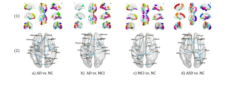 Figure 2. Visualization of discriminative ROIs and connectivity
But the definitive, undeniable evidence that their core mechanism worked wasn't just the high accuracy—it was the Ablation Study and Interpretation Analysis.
When they stripped away the structural mask (reverting the model to a vanilla unimodal Transformer), the accuracy for Alzheimer's classification plummeted by 4.9%. This proved the structural mask wasn't just a gimmick; it was the load-bearing pillar of the model. Furthermore, when they mapped the AI's attention back to the physical brain, the model had independently learned to focus on the precuneus (PCUN) and rectus (REC) for Autism patients—regions that clinical literature has long proven are deactivated when ASD patients attempt to infer mental states. The math didn't just optimize a loss function; it rediscovered biological reality.
Discussion Topics for Future Evolution
Based on this brilliant foundation, here are several deep avenues for future exploration:
- End-to-End Differentiable Structural Sparsity:
Currently, the model relies on XGBoost as a discrete, pre-processing step to extract the structural mask $\mathbf{M}^0$. This breaks the end-to-end differentiability of the pipeline. Could we replace this with a differentiable sparse attention mechanism (like Sparsemax or a Gumbel-Softmax router) that learns to prune the structural graph dynamically during backpropagation? How would this alter the model's ability to discover novel, non-obvious physical biomarkers? - Temporal Dynamics in Functional Connectivity:
This paper treats functional connectivity as a static matrix (Pearson correlation over the whole scan). However, brain activity is highly dynamic; "phone calls" happen in bursts. If we evolve the functional input $\mathbf{X}_f$ into a spatio-temporal sequence and apply a temporal Transformer, how can we mathematically constrain a dynamic functional sequence using a static structural mask? - Cross-Disciplinary Generalization:
The core mathematical premise here—using a static, physical graph to mask and guide attention over a dynamic, functional graph—is not limited to brains. Could this exact architecture be deployed in urban engineering? For example, predicting traffic gridlocks by using the physical road network (structure) to mask attention over real-time GPS movement data (function). What constraints would arise when the "nodes" scale from 90 brain regions to 90,000 city intersections?
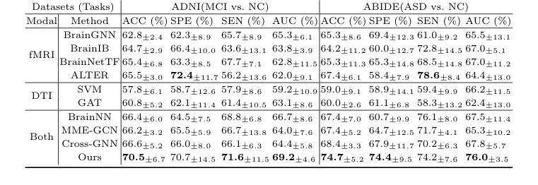 Table 2. Ablation Study Results on Different Datasets
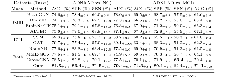 Table 1. Comparative Experiments of Classification Tasks on Different Datasets