Multi-Tube-Voltage vBMD Measurement via Dual-Branch Frequency Balancing and Asymmetric Channel Attention

Background & Academic Lineage

To understand the precise origin of the problem addressed in this paper, we have to look at how doctors diagnose osteoporosis. The gold standard for evaluating bone strength is measuring volumetric Bone Mineral Density (vBMD). Historically, this was done using Quantitative Computed Tomography (QCT), which required placing a physical calibration object—known as a "phantom"—under the patient during the CT scan. The paper notes these physical phantoms are expensive, though to be honest, I'm not completely sure of the exact clinical price tag from the text alone—but in medical imaging, specialized calibration hardware can easily run upwards of \$150 or much more per session, not to mention the hassle of frequent recalibrations.

To bypass this, the medical field developed "phantom-less" (PL) methods. Instead of an external object, these methods use the patient's own internal tissues (like fat and muscle) as reference points to calculate bone density. Recently, Deep Neural Networks (DNNs) have been deployed to automate this process.

However, a massive "pain point" emerged due to a shift in modern clinical practice. To protect patients from excessive radiation, hospitals are increasingly lowering the CT scanner's tube voltage from the standard 120 kVp down to 80 or 100 kVp. The fundamental limitation of previous DNN models is that they were rigidly optimized for 120 kVp scans. When fed lower-voltage images, the overall brightness and contrast (CT attenuation) change drastically. Previous models, relyng heavily on these global intensity changes (low-frequency information), suffer severe performance degradation, producing estimation errors of up to $20 \text{ mg/cm}^3$. They completely miss the fine, spongy textures of the bone (high-frequency information), which actually remain stable regardless of the radiation dose. Furthermore, traditional methods for separating these frequencies are far too computationally heavy to be practical for 3D medical images.

To help you intuitively grasp the science, here are a few highly specialized domain terms translated into everyday concepts:

• Phantom-less (PL) vBMD measurement: Imagine trying to guess the weight of an apple in a photograph. A "phantom" method requires a standard 1-pound metal weight sitting next to the apple for comparison. A "phantom-less" method is like guessing the apple's weight by comparing it to the size of the plate it's sitting on—using what's already in the picture instead of bringing an external tool.
• Tube Voltage (kVp): Think of this as the brightness of a flashlight used to take a photograph. A high voltage (120 kVp) is a blindingly bright light that shows everything clearly but uses a lot of energy (radiation). A lower voltage (80 kVp) is a dimmer light that is safer for the subject but makes the resulting image look different, confusing older computer programs.
• Trabecular architecure: The internal structure of a bone isn't solid rock; it looks more like a rigid sponge or a honeycomb. This term refers to that intricate, porous network inside the bone.
• Frequency decomposition: Imagine listening to a symphony. This process is like using an audio equalizer to separate the deep, booming bass (low-frequency: the overall shape and location of the bone) from the sharp, crisp sounds of the violins (high-frequency: the fine, spongy textures inside the bone).

To solve this, the authors designed a lightweight, dual-branch neural network that separates and balances these frequencies. Mathematically, they extract the high-frequency details without heavy computation and use an asymmetric channel attention mechanism to weigh the importance of each frequency band.

Here is how they mathematically interpret and solve the frequency modulation and feature fusion:

First, they modulate the frequency features using a Fourier transform and a spatial attention mechanism:
$$ Y = \sum_{b \in B} \sigma(f(X_b; W_b)) \odot X_b $$
$$ X_b = \mathcal{F}^{-1}(M_b \odot \mathcal{F}(X)) $$

Later, they fuse the low- and high-frequency features to generate attention weights, ensuring the network focuses on the most critical information:
$$ \widetilde{X} = upsample(X_L) + X_H $$
$$ A_H = \sigma(MLP(GMP(\widetilde{X}))) $$
$$ A_L = \sigma(MLP(GAP(\widetilde{X}))) $$

Finally, they apply these attention weights to decouple the features back into their respective domains:
$$ X = A_H \odot X_H + A_L \odot X_L $$

Below is a table organizing the key mathematical notations necessary to understand their architecture:

Notation	Description
$X$	Input feature map, defined in 3D space as $X \in \mathbb{R}^{C,D,H,W}$
$Y$	Output feature map after frequency modulation
$\mathcal{F}, \mathcal{F}^{-1}$	Fourier transform and its inverse
$M_b$	Binary frequency mask used to isolate specific frequency bands
$W$	Convolutional parameters (weights)
$X_L, X_H$	Decoupled low-frequency and high-frequency feature componets
$Y_L, Y_H$	Processed low-frequency and high-frequency features
$A_L, A_H$	Channel attention maps for low and high frequencies
$\widetilde{X}$	Fused feature map before re-splitting
$AP(x)$	Average pooling operation with a $2 \times 2 \times 2$ kernel
$upsample(x)$	Nearest neighbor upsampling operation
$\sigma$	Sigmoid activation function
$\odot$	Hadamard product (element-wise multiplication)

Problem Definition & Constraints

Imagine you are trying to weigh a sponge, but instead of putting it on a scale, you have to guess its weight just by looking at a photograph of it. Now, imagine the lighting in the room keeps changing—sometimes it's bright, sometimes it's dim. This is exactly the challenge doctors face when trying to measure bone density from CT scans without using a physical calibration tool (a "phantom").

The Starting Point and the Desired Endpoint

The Input (Current State): We start with 3D Computed Tomography (CT) images of a patient's vertebral bodies. These scans are taken at varying radiation levels, known as tube voltages (typically 80, 100, or 120 kVp).

The Output (Goal State): The goal is to output a highly accurate volumetric Bone Mineral Density (vBMD) measurement, expressed in $mg/cm^3$.

The Mathematical Gap:
Traditionally, doctors measure bone density by looking at the Hounsfield Unit (HU), which is a mathematical representation of how much the tissue blocks X-rays. The missing link here is that HU values are strictly dependent on the X-ray tube voltage. If a hospital lowers the voltage to save the patient from excess radiation, the HU values of the exact same bone will drop significantly. The authors needed to build a mathematical bridge that maps a highly variable, voltage-dependent 3D spatial intensity matrix $X \in \mathbb{R}^{C,D,H,W}$ into a stable, absolute density value, completely independent of the scanner's settings.

The Painful Dilemma

In the world of computer vision, improving one aspect almost always breaks another. For this specific problem, previous researchers have been trapped in a brutal trade-off between frequency extraction and computional cost.

To understand this, we have to split an image into two "frequencies":
1. Low-frequency features: The broad, macroscopic shapes (like the overall outline of the spine). These are easy for standard neural networks to learn and help the model quickly locate the bone. However, they are highly sensitive to tube voltage changes.
2. High-frequency features: The tiny, fine-grained, sponge-like micro-architecure of the bone (the trabecular structure). These features are incredibly stable across different voltages and are the true indicators of osteoporosis.

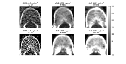Figure 1. Intuitive comparison of features in vBMD measurement. The first row shows vertebral bodies with varying bone densities at 120 kVp. The second row shows corresponding vertebral bodies at non-120 kVp, where vBMD texture remains similar, but HU values within the VOI differ significantly. Low vBMD vertebral bodies exhibit both reduced HU values and a sparser trabecular structure in the measurement area

Here is the dilemma: Standard Deep Neural Networks (DNNs) naturally prioritize low-frequency information. If you want to force a network to pay attention to high-frequency 3D textures, you traditionally have to use deep, complex networks or heavy mathematical operations like 3D wavelet transforms. But doing this in 3D space causes an exponential explosion in memory and processing requirements. You either get a lightweight model that fails when the hospital changes the CT voltage, or a robust model that is too massive and slow to run on standard clinical hardware.

The Harsh Walls and Constraints

The authors hit several harsh, realistic walls that make this problem insanely difficult to solve:

• The Clinical Radiation Wall: There is a massive global push to lower radiation exposure for patients, dropping scans from 120 kVp down to 80 kVp. At these lower voltages, global intensity measures become fundamentally un-relyable. The model must adapt to these darker, lower-energy scans without losing accuracy.
• The Physical Sparsity of the Disease: Osteoporosis is literally the vanishing of bone. As the disease progresses, the trabecular bone becomes extremely sparse. The network is forced to look for microscopic textural features that are actively disappearing.
• The 3D Computational Bottleneck: Medical images are not flat 2D pictures; they are massive 3D volumes. Applying traditional frequency decomposition (like repeated Fourier transforms) across depth, height, and width requires immense memory. The authors had to find a way to decouple frequencies without heavy math, opting instead for a clever trick using average pooling to extract low frequencies, and subtracting that from the original image to find the high frequencies.
• The Feature Mixing Trap: If you try to process low and high frequencies in parallel (a dual-branch network), standard convolution layers tend to accidentally mix the information back together. The authors had to design a strict mathematical gatekeeper—an asymmetric channel attention mechanism—to ensure the high-frequency branch only looked at the fine details and the low-frequency branch only looked at the broad shapes. This is defined mathematically by separating the feature map $X$ into its low-frequency ($X_L$) and high-frequency ($X_H$) components:
  $$X = upsample(X_L) + X_H$$

In short, the authors had to build a system that could see the microscopic, disappearing structure of a bone in 3D, ignore the changing "lighting" of the X-ray machine, and do it all on a strict computational budget.

Why This Approach

The exact moment the authors realized that traditional state-of-the-art (SOTA) methods—such as standard 3D Convolutional Neural Networks (CNNs), Vision Transformers, or Diffusion models—were fundamentally insufficient for this problem occurred when they analyzed the physical behavior of CT scans under varying tube voltages. To reduce radiation exposure, modern clinics often lower CT tube voltages from the standard $120$ kVp down to $100$ kVp or $80$ kVp. However, this drop in voltage drastically alters the global Hounsfield Unit (HU) values (the standard measure of radiodensity). Standard CNNs naturally prioritize low-frequency information, which corresponds to the overall shape and global intensity of the image. Because these low-frequency global intensities are highly sensitive to voltage changes, a standard model trained on $120$ kVp data experiences massive performance degradation when tested on $80$ kVp data, yielding errors up to $20$ $mg/cm^3$.

The authors had a crucial realization: while the global intensity shifts with voltage, the high-frequency features—specifically, the fine, sponge-like trabecular micro-architecure of the bone—remain structurally stable. Therefore, any standard network that blurs out high-frequency textural details in favor of macroscopic shapes was doomed to fail. They absolutely had to process these frequency domains separately.

Beyond simple performance metrics, this method is qualitatively superior because of how it handles the immense computional burden of 3D medical imaging. Traditional frequency-domain methods typically rely on computationally intensive techniques like wavelet transforms or multi-scale convolution kernels to separate frequencies. If applied to massive 3D volumetric CT data, the memory complexity would skyrocket, making the models practically unusable in clinical settings. The authors achieved a massive structural advantage by abandoning heavy mathematical transforms at every layer. Instead, they introduced a brilliantly simple decoupling method: they extract the low-frequency components ($X_L$) using average pooling to downscale the feature map, and then derive the high-frequency components ($X_H$) by simply calculating the residual between the original feature map and the upsampled low-frequency map. Mathematically, this is expressed as:

$$X_H = X - \text{upsample}(X_L)$$

This elegantly bypasses the need for heavy signal processing. Furthermore, instead of applying Fourier transforms repeatedly throughout the network—which creates massive overhead—they restrict frequency modulation to the shallow layers where local feature extraction is most critical.

This chosen architecture represents a perfect "marriage" between the problem's harsh constraints and the solution's unique properties. The constraints dictate that the model must generalize across varying CT tube voltages without relyng on external calibration phantoms, while simultaneously processing heavy 3D data efficiently. The dual-branch architecture perfectly aligns with this. By splitting the network, the model uses a deeper pathway to understand the macroscopic vertebral anatomy (low frequency) and a shallower pathway to capture the delicate trabecular structures (high frequency). To fuse them, they utilize an asymmetric channel attention mechanism. They apply Global Max Pooling (GMP) to highlight the sharp, stable high-frequency details, and Global Average Pooling (GAP) for the smooth low-frequency data:

$$A_H = \sigma(MLP(GMP(\tilde{X})))$$
$$A_L = \sigma(MLP(GAP(\tilde{X})))$$

This ensures that the stable trabecular features actively guide the final volumetric Bone Mineral Density (vBMD) measurement, making the model incredibly robust against voltage-induced intensity shifts.

Finally, this explains why other popular approaches, such as Generative Adversarial Networks (GANs) or Diffusion models, would have catastrophically failed here. Generative models are designed to synthesize or hallucinate missing data distributions. In quantitative medical imaging, where exact physical measurements are required to diagnose osteoporosis, hallucinating structural data is clinically dangerous. Furthermore, these models are notoriously heavy. The authors explicitly note that even extending standard 2D DNNs to 3D requires "excessive computational resources." Deploying a massive Transformer or a multi-step Diffusion process for 3D volumetric CT scans would be computationally paralyzing and entirely unnecessary for a regression task aimed at extracting stable structural textures. The lightweight, frequency-balancing dual-branch network was the only viable path that satisfied both the clinical demand for absolute precision and the engineering demand for efficiency.

Mathematical & Logical Mechanism

To understand the core of this paper, we first need to understand the physical problem it solves. When doctors measure volumetric Bone Mineral Density (vBMD) using CT scans, they usually rely on a specific radiation tube voltage, typically 120 kVp. However, modern clinics are shifting to lower voltages (like 80 or 100 kVp) to reduce radiation exposure to patients. The problem? Lowering the voltage drastically changes the overall brightness and contrast (Hounsfield Units) of the CT image.

If a deep learning model memorizes the overall brightness (low-frequency data) at 120 kVp, it will fail miserably at 80 kVp. However, the fine, sponge-like trabecular structure of the bone (high-frequency data) remains physically stable regardless of the voltage. The authors designed a brilliant dual-branch neural network that splits the image into low and high frequencies, dynamically weighs their importance, and fuses them back together.

Here is the absolute core mathematical engine that makes this cross-voltage generalization possible.

$$ \widetilde{X}_{base} = upsample(X_L) + X_H $$
$$ A_H = \sigma(MLP(GMP(\widetilde{X}_{base}))) $$
$$ A_L = \sigma(MLP(GAP(\widetilde{X}_{base}))) $$
$$ \widetilde{X}_{coupled} = A_H \odot X_H + A_L \odot X_L $$
$$ Y_L = AP(\widetilde{X}_{coupled}) $$
$$ Y_H = \widetilde{X}_{coupled} - upsample(Y_L) $$

(Note: The authors use $\widetilde{X}$ to represent both the initial fused state and the attention-coupled state. I have added the subscripts 'base' and 'coupled' to make the chronological transformation clearer).

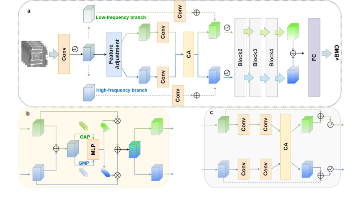Figure 2. The proposed network. The proposed network adopts a dual-branch ar- chitecture consisting of four distinct modules (a). The first module is responsible for spatial reallocation of feature maps in the frequency domain. The following modules incorporate convolutional layers designed to perform coupling and re-decoupling oper- ations, guided by a channel attention mechanism (b and c). This design facilitates the effective fusion of frequency features, thereby enhancing the model’s ability to dynam- ically process both low- and high-frequency information.CA, channel attention; FC, fully connected

Let's tear this engine apart piece by piece to see how it ticks.

• $X_L$ and $X_H$: These are the input feature maps for the Low-frequency and High-frequency branches. $X_L$ represents the macroscopic, blurry shape of the bone (highly sensitive to voltage changes). $X_H$ represents the sharp, fine-grained trabecular mesh (stable across voltages).
• $upsample()$: A nearest-neighbor upsampling function. Because low-frequency features are often pooled and downscaled to save memory, they must be stretched back to the same spatial dimmension as the high-frequency features before they can interact.
• $+$ (Addition): Why add instead of concatenate? Concatenation would double the memory footprint. Addition acts as a physical superposition—like adding a sharp texture map directly on top of a blurry color map in the same mathematical space.
• $GMP()$ and $GAP()$: Global Max Pooling and Global Average Pooling. This is where the physics of the bone comes into play. $GMP$ acts as a radar for the absolute sharpest, highest-intensity spikes (perfect for isolating the hard trabecular bone structure). $GAP$ calculates the overall ambient energy or average density of the region.
• $MLP()$: A Multi-Layer Perceptron (a small neural network). This acts as the "brain" that looks at the pooled statistics and decides which specific feature channels are actually useful for predicting bone density.
• $\sigma$ (Sigmoid Function): This squashes the output of the MLP into a range between 0 and 1. It acts as a set of dimmer switches.
• $A_H$ and $A_L$: The resulting Attention weights for the high and low frequencies.
• $\odot$ (Hadamard Product): Element-wise multiplication. Why multiplication here instead of addition? Because this is a gating mechanism. If a specific low-frequency channel is deemed too corrupted by a voltage change, its corresponding $A_L$ value might be 0.1, effectively muting that channel. If a high-frequency channel contains vital structural data, its $A_H$ might be 0.9, amplifying it.
• $AP()$: Average Pooling with a $2 \times 2 \times 2$ kernel. This acts as a low-pass filter, smoothing out the newly coupled master feature map to extract the refined low-frequency output, $Y_L$.
• $-$ (Subtraction): Why subtraction to get $Y_H$? This is a beautiful use of residual logic. High frequency is mathematically defined as "everything that is not low frequency." By subtracting the smoothed base ($upsample(Y_L)$) from the master coupled map ($\widetilde{X}_{coupled}$), the network perfectly isolates the crisp, high-frequency details without needing complex, computationally heavy Fourier transforms at this stage.

Step-by-step Flow

Imagine a 3D block of raw CT data entering a mechanical assembly line.

First, the data is split onto two separate conveyor belts: one carrying the blurry, overall bone shape ($X_L$) and the other carrying the sharp, sponge-like bone texture ($X_H$). The blurry shape is physically stretched ($upsample$) to match the exact size of the sharp texture, and the two are stacked on top of each other to create a composite block ($\widetilde{X}_{base}$).

Next, this composite block passes under two specialized sensors. The first sensor ($GMP$) scans for the sharpest, most extreme structural spikes. The second sensor ($GAP$) measures the overall ambient density. These readings are fed into a central computer ($MLP$), which calculates exactly how reliable each feature channel is.

The computer outputs two sets of dials ($A_H$ and $A_L$). These dials are applied back to the original conveyor belts, dimming the irrelevant or noisy channels and boosting the highly relevent ones. The optimized belts are then merged into a master, coupled block ($\widetilde{X}_{coupled}$).

Finally, this master block is pressed through a smoothing machine ($AP$) to create a newly refined, stable blurry shape ($Y_L$). To get the refined sharp texture ($Y_H$), the machine simply takes the master block and slices away the blurry shape ($-$). The two perfectly balanced, updated components then move forward to the next stage of the architecure.

Optimization Dynamics

How does this mechanism actually learn and converge? The network is trained end-to-end using a regression loss (like Mean Absolute Error) against gold-standard, phantom-based measurements taken at 120 kVp.

Because the architecture relies heavily on addition and subtraction, the loss landscape is remarkably smooth. In calculus, the local derivative of an addition or subtraction operation is exactly 1 (or -1). This means that when the network makes an error, the gradient signal flows backward through the $Y_H$ and $Y_L$ equations without degrading or vanishing.

As training progresses, the $MLP$ receives continuous feedback. If the model overestimates bone density because it relied too heavily on a low-frequency channel that was artificially darkened by an 80 kVp scan, the gradient tells the $MLP$: "Next time you see this specific variance, turn down the $A_L$ dimmer switch." Over time, the network learns to dynamically shift its attention. When it detects the confusing global intensity shifts of low-voltage scans, it automatically relies more heavily on the stable, high-frequency trabecular features.

To be honest, I'm not completely sure exactly which specific optimizer (e.g., Adam, SGD) or learning rate schedule the authors used, as those hyperparameter details aren't explicitly listed in the provided text. However, the structural design itself—specifically the residual decoupling and asymmetric attention—acts as a natural regularizer. It prevents the model from overfitting to the absolute Hounsfield Units of any single tube voltage, forcing it to learn the underlying physical reality of the bone instead.

Results, Limitations & Conclusion

Imagine you are trying to determine the structural integrity of a building, but you are only allowed to look at photographs of it. To make things harder, some photos are taken in bright daylight, while others are taken at dusk with a cheap camera. The overall color and brightness of the building change drastically depending on the lighting, but the fine cracks in the concrete—the high-frequency details—remain consistent.

This is exactly the problem doctors face when measuring Volumetric Bone Mineral Density (vBMD) to diagnose osteoporosis using Computed Tomography (CT) scans.

Historically, hospitals used physical calibration objects called "phantoms" (which can be quite expensive, sometimes adding the equivalent of USD 150 or more to procedure overheads) placed under the patient during a scan to provide a baseline density reference. To cut costs, "phantom-less" (PL) methods were developed, using the patient's own fat and muscle as reference points. However, a massive constraint emerged: modern clinics are lowering the radiation dose of CT scans (dropping the tube voltage from 120 kVp down to 80 or 100 kVp) to protect patients. This fundemental shift alters the Hounsfield Units (the pixel intensity values in a CT scan). Traditional AI models, which rely heavily on the "big picture" overall brightness (low-frequency data), get completely confused by this voltage drop, leading to massive measurement errors.

The authors of this paper realized something brilliant: while the overall brightness of the bone changes with lower radiation, the microscopic, sponge-like texture of the bone (the trabecular structure) does not. They needed an AI that could ignore the shifting lighting and focus on the cracks in the concrete.

The Mathematical Core: Decoupling and Modulating Reality

To solve this, the authors had to overcome a severe computational constraint. Extracting high-frequency 3D textures usually requires incredibly heavy math, like multi-scale wavelet transforms, which would crash standard hospital computers.

Instead, they designed a lightweight, dual-branch network that splits the image into seperate pathways. First, they extract the low-frequency "blurry" data ($X_L$) using a simple average pooling operation. Then, they subtract this blurry image from the original to isolate the high-frequency "sharp" details ($X_H$).

To ensure the network pays attention to these sharp details early on without bogging down the system, they apply a frequency domain modulation using Fourier transforms ($\mathcal{F}$). Mathematically, they selectively enhance the high-frequency features using a spatial attention mechanism:

$$Y = \sum_{b \in B} \sigma(f(X_b; W_b)) \odot X_b$$

where the frequency bands are isolated via:

$$X_b = \mathcal{F}^{-1}(M_b \odot \mathcal{F}(X))$$

Here, $M_b$ is a binary mask that filters the frequencies, and $\odot$ represents the Hadamard (element-wise) product.

Once the features are modulated, they are sent down two distinct convolutional branches:

$$Y_L = f(X_L; W_L) + X_L$$
$$Y_H = f(X_H; W_H) + X_H$$

But the true genius lies in how they fuse these branches back together. They don't just mash them up at the end. They use an asymmetric channel attention mechanism. For the high-frequency data, they use Global Max Pooling (GMP) because max pooling is excellent at detecting sharp, isolated spikes (like the edge of a bone trabecula). For the low-frequency data, they use Global Average Pooling (GAP) to capture the general, smooth anatomical layout.

They calculate attention weights ($A_H$ and $A_L$) to decide how important each feature is:

$$\widetilde{X} = upsample(X_L) + X_H$$
$$A_H = \sigma(MLP(GMP(\widetilde{X})))$$
$$A_L = \sigma(MLP(GAP(\widetilde{X})))$$

Finally, they re-split the data, applying these learned weights to ensure the network maintains a perfect balance of macroscopic anatomy and microscopic texture:

$$X = A_H \odot X_H + A_L \odot X_L$$

The Experimental Architecure: A Ruthless Proof

The authors didn't just throw their model at a clean dataset and claim a 5% accuracy bump. They architected an experiment designed to ruthlessly test their mathematical claims against the chaotic reality of clinical environments.

They gathered data from two entirely independent medical centers. One center's data was used to train and internally test the model (1,614 images), while the other center's data (2,245 images) was kept in a locked vault as an "external testing set." This ensures the AI didn't just memorize the specific quirks of one hospital's CT scanner.

The Victims:
The authors pitted their creation against three baselines:
1. A traditional Phantom-less (PL) linear regression method (adapted with a mathematical conversion formula to try and handle multi-voltage data).
2. ResNet-10 (a standard, highly respected deep learning model).
3. OctResNet-10 (a model specifically designed to handle spatial redundancy).

The Undeniable Evidence:
The definitive proof that their core mechanism worked wasn't just in beating the victims across 120 kVp and 100 kVp datasets (achieving a highly superior Mean Absolute Error of 5.990 $mg/cm^3$ internally and 7.175 $mg/cm^3$ externally). The real smoking gun was their Ablation Study.

They systematically lobotomized their own model. They turned off the frequency balancing. Then they turned off the channel attention. In every case, the error rates spiked. It was only when both the high/low-frequency decoupling and the asymmetric GMP/GAP attention mechanisms were working in tandem that the model achieved its peak performance. This proved mathematically and empirically that their hypothesis was correct: you must isolate and uniquely weight high-frequency textures to survive tube voltage variations.

To be honest, I'm not completely sure about the exact physical physics causing the severe image degradation at the 80 kVp level in the external dataset—the authors note their model underperformed the baseline there due to "significant image quality differences across centers," which suggests that at extremely low radiation, the high-frequency trabecular data might simply be destroyed by quantum noise before the AI can even see it.

Discussion Topics for Future Evolution

Based on the profound implications of this paper, here are several avenues for future exploration and critical thought:

1. The Threshold of Information Destruction:
   At 80 kVp, the model struggled on external data. This raises a fascinating physics-meets-AI question: At what exact radiation dose does the high-frequency trabecular structure transition from "hidden but recoverable" to "physically destroyed by photon starvation and quantum noise"? Can we mathematically define the absolute lower bound of radiation required for AI-driven bone density analysis?

2. Cross-Modality Frequency Decoupling:
   If separating high-frequency textures from low-frequency global illumination solves the CT voltage problem, could this exact mathematical framework be ported to MRI or Ultrasound? For instance, could this dual-branch architecture isolate the high-frequency micro-tears in ligaments on an MRI, ignoring the low-frequency variations caused by different magnetic field strengths (1.5T vs 3T)?

3. The End of Physical Phantoms?
   The economic implications here are massive. If software can reliably dynamically adjust to any scanner's voltage using internal tissue references and frequency modulation, do we ever need to manufacture, ship, and calibrate physical CT phantoms again? What are the regulatory and legal hurdles of replacing a physical ground-truth object with a probabilistic neural network in life-or-death diagnostic scenarios?

Isomorphisms with other fields

To understand this paper, we first need to look at how doctors diagnose osteoporosis. They measure volumetric Bone Mineral Density (vBMD) using CT scans. Traditionally, this requires a "phantom"—a physical calibration object placed under the patient during the scan, which is expensive and cumbersome. Phantom-less (PL) methods use the patient's own internal tissues (like fat and muscle) as reference points instead.

The motivation stems from a critical constraint in modern hospitals: varying radiation doses. To save patients from excessive radiation, clinics increasingly use lower tube voltages (like 80 kVp or 100 kVp instead of the standard 120 kVp). The problem is that lowering the voltage drastically alters the global pixel intensities (Hounsfield Units, or HU) of the CT image. Because existing deep learning models rely heavily on these low-frequency global intensities, their accuracy collapses when the voltage drops. However, the authors noticed a crucial biological loophole: while the overall brightness changes, the high-frequency texture of the spongy trabecular bone remains remarkably stable across different voltages.

To solve this, the authors needed to mathematically decouple the volatile macroscopic data from the stable microscopic data. Instead of feeding the whole image into a standard neural network, they built a dual-branch architecture to seperate the frequencies.

First, they modulate the frequency features using a Fourier transform paired with spatial attention to avoid redundant computational overhead. For an input feature map $X$, the modulated output $Y$ is defined as:

$$ Y = \sum_{b \in B} \sigma(f(X_b; W_b)) \odot X_b $$

where the frequency bands are extracted via $X_b = \mathcal{F}^{-1}(M_b \odot \mathcal{F}(X))$, with $\mathcal{F}$ representing the Fourier transform and $M_b$ acting as a binary frequency mask.

Once the signal is split into low-frequency ($X_L$) and high-frequency ($X_H$) components, they are processed in parallel branches. The true genius of the paper lies in how these branches are fused back together. The authors recognized that high-frequency data (sharp bone edges) and low-frequency data (general bone shape) require different mathematical lenses. They designed an asymmetric channel attention mechanism. They apply Global Max Pooling (GMP) to capture the sharp peaks of high-frequency features, and Global Average Pooling (GAP) to smooth and capture the low-frequency features:

$$ A_H = \sigma(MLP(GMP(\tilde{X}))) $$
$$ A_L = \sigma(MLP(GAP(\tilde{X}))) $$

These attention weights are then used to dynamically recombine the decoupled signals:

$$ \tilde{X} = A_H \odot X_H + A_L \odot X_L $$

This equation allows the network to adaptively trust the stable high-frequency texture when the low-frequency global intensity becomes unreliable due to voltage changes.

At its core, the structural skeleton of this work is a mechanism that isolates a complex signal into volatile macroscopic baselines and stable microscopic fluctuations, processes them in parallel, and dynamically recombines them using an asymmetric weighting function to extract an invariant metric across varying enviornmental conditions.

Based on this skeleton, we can find "Mirror Images" of this exact logic in completely different fields of science and engineering:

1) Quantitative Finance: In algorithmic trading, asset prices consist of macroeconomic trends (low-frequency, highly sensitive to external "voltages" like interest rate hikes) and micro-structural order book dynamics (high-frequency, representing the stable, intrinsic trading behavior). Extracting the true fundemental value of an asset by decoupling market-wide noise from intrinsic micro-volatility is a direct mirror of separating CT global intensity from trabecular texture.
2) Seismology: When detecting the magnitude of an earthquake, seismographs record low-frequency surface waves (which are heavily distorted by the local soil type, acting like varying CT tube voltages) and high-frequency body waves (which carry the true, stable signature of the fault line's rupture). Seismologists constantly struggle to balance these frequencies to find the invariant truth of the quake.

What would happen if a quantitative finance researcher "stole" this paper's exact asymmetric attention equation tomorrow? If they applied $$ \tilde{X} = A_H \odot X_H + A_L \odot X_L $$ to a high-frequency trading algorithm, they could use Global Max Pooling to aggressively capture the absolute peaks of order-book anomalies (the "trabecular" trades) while using Global Average Pooling to smooth out the volatile macroeconomic sentiment. The breakthrough would be a radically robust trading bot that maintains its predictive accuracy and profitability regardless of whether the broader market suddenly shifts into a high-volatility or low-volatility regime—effectively making the algorithm immune to market "tube voltage" fluctuations.

Ultimately, this architecture proves that whether we are measuring the density of decaying bone or the hidden value of a fluctuating financial asset, the mathematical pursuit of invariant truth relies on the exact same symphony of decoupled frequencies and adaptive attention, adding a brilliant new blueprint to the Universal Library of Structures.

---