Energy-Guided Continuous Entropic Barycenter Estimation for General Costs

Background & Academic Lineage

The Origin & Academic Lineage

The problem addressed in this paper, the Optimal Transport (OT) barycenter problem, arises from the fundamental need to average probability distributions in a geometrically meaningful way. While averaging scalars or vectors in linear spaces is straightforward, the task becomes significantly more complex when dealing with probability distributions. Simple convex combinations often fail to preserve essential geometric features, necessitating a more sophisticated approach to define a "center" or average.

This specific problem first emerged in the academic field of Optimal Transport, which provides a robust framework for comparing and averaging probability distributions by defining a "cost" to transform one distribution into another. The concept of OT barycenters, introduced by Agueh and Carlier [1] in 2011, seeks to find a central distribution that minimizes the sum of transport costs to a given collection of source distributions.

Over the last decade, the practical demand for effective barycenter computation has driven substantial research. Initial efforts primarily focused on the discrete OT barycenter setting, where distributions are represented by finite sets of points. However, the continuous setting, which deals with continuous probability distributions, proved to be far more challenging. Previous continuous OT barycenter solvers suffered from several key limitations:

1. Specific Cost Functions: Many existing methods were designed exclusively for specific OT cost functions, most notably the quadratic Euclidean cost ($l_2(x, y) \stackrel{\text{def}}{=} ||x - y||^2$). This restricted their applicability to a narrow range of problems, as real-world scenarios often involve non-Euclidean or more complex cost functions.
2. Non-trivial a priori Selections: Some approaches required intricate a priori selections or fixed priors for the barycenter distribution, which could be non-trivial to determine and might limit the model's flexibility.
3. Limiting Expressivity and Generative Ability: Certain methods had limited capacity to express complex relationships between distributions or to generate new samples from the learned barycenter, hindering their utility in generative modeling tasks.
4. Inability to Recover OT Plans: Some approaches parameterized the barycenter as a generative model but did not recover the underlying Optimal Transport plans, which are crucial for understanding how individual source distributions map to the barycenter.

This paper aims to overcome these limitations by proposing a novel algorithm for approximating the continuous Entropic OT (EOT) barycenter that can handle arbitrary OT cost functions, without requiring fixed priors or limiting expressivity, and importantly, it recovers the conditional OT plans.

Intuitive Domain Terms

To help a zero-base reader grasp the core concepts, here are some specialized terms translated into everyday analogies:

• Optimal Transport (OT): Imagine you have several piles of dirt (probability distributions) and you want to reshape them into a new pile. Optimal Transport is like finding the most efficient way to move all the dirt from the original piles to form the new one, minimizing the total "work" or "cost" involved.
• Barycenter: If you have several scattered clouds of smoke (probability distributions), the barycenter is like finding the "average" or "center of mass" smoke cloud that is, on average, closest to all the original clouds, considering the "effort" (Optimal Transport cost) to transform one cloud into another. It's the central point that balances the "pull" from all the other distributions.
• Entropic Optimal Transport (EOT): This is a "softer" or "fuzzier" version of Optimal Transport. Instead of strictly moving every particle of dirt along the most direct path, EOT allows for a little bit of mixing or randomness during the transport. This makes the problem easier to solve computationally, like allowing some dirt to spread a little, while still achieving a good, geometrically sensible average.
• Weak OT Dual Formulation: Think of a complex problem, like designing the perfect bridge. Instead of directly building and testing every possible bridge, a "dual formulation" is like finding a simpler, equivalent problem that involves optimizing the forces and stresses on the bridge. In OT, it means we don't directly track every "dirt particle" but instead find two "potential functions" that, when optimized, indirectly tell us the most efficient way to move the dirt. This is often easier to solve.
• Energy-Based Models (EBMs): Imagine a landscape where valleys represent places data points are likely to be, and hills represent unlikely places. EBMs learn this "energy landscape" to understand how data is distributed. Our method uses a similar idea: it frames the barycenter problem as finding the lowest "energy" configuration in a complex space, allowing us to leverage well-established EBM training techniques to find the solution.

Notation Table

Notation	Description

Problem Definition & Constraints

Core Problem Formulation & The Dilemma

The core problem addressed by this paper is the estimation of the continuous Entropic Optimal Transport (EOT) barycenter for a collection of probability distributions.

Input/Current State:
The starting point involves a collection of $K$ source probability distributions, denoted as $P_k \in \mathcal{P}_{ac}(\mathcal{X}_k)$, where $\mathcal{P}_{ac}(\mathcal{X}_k)$ represents absolutely continuous probability distributions defined on compact subsets $\mathcal{X}_k \subset \mathbb{R}^{D_k}$. For each source distribution $P_k$, there is an associated continuous cost function $c_k(\cdot, \cdot) : \mathcal{X}_k \times \mathcal{Y} \to \mathbb{R}$, which quantifies the "cost" of transporting mass between points in $\mathcal{X}_k$ and points in the barycenter space $\mathcal{Y}$. Additionally, a set of positive weights $\lambda_k > 0$ are given, satisfying the condition $\sum_{k=1}^K \lambda_k = 1$. Crucially, in practical scenarios, these source distributions $P_k$ are not explicitly known but are only accessible through finite sets of empirical samples, $X_k = \{x_1^k, x_2^k, \dots, x_{N_k}^k\} \sim P_k$. Existing continuous OT barycenter solvers often struggle with general cost functions, require specific a priori selections, or have limited expressivity and generative capabilities.

Desired Endpoint (Output/Goal State):
The ultimate goal is to identify the EOT barycenter $Q^* \in \mathcal{P}(\mathcal{Y})$, which is a probability distribution that minimizes the weighted sum of EOT discrepancies to all source distributions $P_k$. Mathematically, this is formulated as:
$$L^* \stackrel{\text{def}}{=} \inf_{Q \in \mathcal{P}(\mathcal{Y})} \sum_{k=1}^K \lambda_k \text{EOT}_{c_k, \epsilon}(P_k, Q)$$
Here, $\text{EOT}_{c_k, \epsilon}(P_k, Q)$ represents the entropic optimal transport cost between $P_k$ and $Q$, regularized by a parameter $\epsilon > 0$. Beyond just finding $Q^*$, the paper aims to approximate the optimal conditional transport plans $\pi_{f_k}^*(\cdot|x_k)$ that map points from each source $P_k$ to the barycenter $Q^*$. These recovered plans should enable "out-of-sample estimation," meaning they can generate samples from $\pi_{f_k}^*(\cdot|x_{\text{new}})$ for new, unseen samples $x_{\text{new}}$ from $P_k$. A further ambition is to learn the barycenter on a pre-trained generative model's image manifold, which has significant implications for real-world applications.

Missing Link & The Dilemma:
The exact missing link is a general, robust, and computationally feasible algorithm for estimating continuous EOT barycenters that can handle arbitrary cost functions and operate effectively with only empirical samples from the source distributions. Previous research has been trapped by a painful trade-off: achieving greater generality and expressivity in continuous OT barycenter problems typically introduces significant computational challenges or requires restrictive assumptions. For instance, improving generality to handle arbitrary cost functions often leads to intractable optimization problems, as many prior methods rely on specific, simpler costs (like the quadratic Euclidean $l_2$ cost) due to their advantageous theoretical properties. These simpler costs allow for more efficient algorithms, but limit applicability. Furthermore, while the continuous setting is more powerful, it is also "even more challenging" than the discrete setting, with existing solutions often having limitations in expressivity or requiring non-trivial a priori selections or specific parametrizations of the barycenter, which can be difficult to determine or limit the method's scope. Another dilemma arises in high-dimensional data spaces, such as images: direct computation of EOT barycenters often results in "noisy images" or "blurring bias" due to entropy regularization and reliance on MCMC. While restricting the search space to a data manifold can mitigate this, it introduces its own set of complexities related to manifold learning and adaptation of cost functions.

Constraints & Failure Modes

The problem of continuous EOT barycenter estimation is inherently difficult due to several harsh, realistic constraints:

1. Computational Intractability of Direct Optimization: The objective function for the EOT barycenter (Equation 5) involves an $\inf$ over the space of all probability distributions $\mathcal{P}(\mathcal{Y})$, which is an infinite-dimensional space. Directly optimizing this is generally intractable, necessitating a reformulation of the problem.
2. Lack of Analytical Solutions: For most practical scenarios, including cases with Gaussian distributions, there is no known direct analytical solution for the entropic barycenter problem (both for $\epsilon > 0$ and the unregularized $\epsilon = 0$ case). This forces reliance on numerical approximation methods.
3. Empirical Data Limitation: Source distributions $P_k$ are rarely available explicitly in real-world applications. Instead, only finite empirical samples (datasets) $X_k$ are accessible. This means algorithms must be robust to data sparsity and noise, and capable of out-of-sample generalization.
4. High-Dimensionality: Working with complex data types, such as RGB images (e.g., $3 \times 64 \times 64$ dimensions for CelebA), introduces significant computational and memory demands for learning and sampling, making direct approaches infeasible.
5. Arbitrary Cost Functions: The paper aims to support "arbitrary OT cost functions," which is a substantial constraint. Many existing methods are specialized for simpler costs (like $l_2$), which possess specific theoretical properties that simplify computation. General costs remove these simplifications, increasing complexity.
6. Non-Euclidean Geometries: The problem explicitly considers "non-Euclidean cost functions," meaning standard Euclidean distance metrics are often inadequate. This requires more flexible and powerful models to capture complex geometric relationships.
7. MCMC Sampling Limitations: The proposed method relies on Markov Chain Monte Carlo (MCMC) procedures (specifically Unadjusted Langevin Algorithm, ULA) for sampling.
   • High Computational Cost: MCMC sampling is inherently "time-consuming," impacting training and inference latency (Table 3).
   • Convergence Issues: The basic ULA algorithm "may poorly converge to the desired distribution," leading to suboptimal results.
   • Differentiability Requirement: MCMC typically requires the energy functions (and thus the cost functions $c_k$) to be differentiable. Non-differentiable costs would necessitate more complex, gradient-free sampling procedures.
   • Local Minima: MCMC inference can get "stuck in local minima of the energy landscape," causing the learned transport plans to fail in preserving desired image content or other features (Section 5.3).
8. Infeasible Normalizing Constant: The direct computation of the normalizing constant $Z_{c_k}(f_k, x_k)$ within the dual objective function is often "infeasible," requiring approximations for gradient estimation.
9. "Blurring Bias" in Data Space: When EOT barycenters are computed directly in high-dimensional data spaces (e.g., image pixels), the entropy regularization can lead to "noisy images" or a "blurring bias," making the resulting barycenter less interpretable or visually plausible.
10. Manifold Constraint Complexity: While restricting the barycenter search to a data manifold (e.g., using a pre-trained StyleGAN) helps mitigate blurring, it introduces the additional complexity of training and integrating such generative models, and adapting cost functions to the latent space of the manifold.
11. Generalization and Approximation Errors: Ensuring that the learned models generalize well to unseen data and that neural network approximations are accurate is a significant theoretical challenge. The estimation error can suffer from the "curse of dimensionality" for general Lipschitz costs, making it difficult to achieve fast convergence rates in high dimensions.

Why This Approach

The Inevitability of the Choice

The authors' choice of an Energy-Guided Continuous Entropic Barycenter Estimation approach was not merely a preference but a necessity driven by the inherent limitations of existing methods for continuous Optimal Transport (OT) barycenter problems. The exact moment of this realization is evident from the detailed discussion in Section 3 and Table 1, which highlight the shortcomings of prior art.

Traditional "SOTA" methods, such as standard CNNs, basic Diffusion models, or Transformers, were deemed insufficient because:
1. Specific Cost Functions: A significant portion of previous continuous OT solvers, including works like [59, 55, 32, 82], were designed exclusively for the quadratic Euclidean cost $l_2(x, y) = ||x - y||^2$. This limitation severely restricts their applicability to real-world scenarios where arbitrary, non-Euclidean cost functions are essential for capturing complex geometric relationships between distributions. The paper explicitly states, "In contrast, our proposed approach is designed to handle the EOT problem with arbitrary cost functions $c_1, \dots, c_K$." (page 4).
2. Fixed Priors and Non-trivial Selections: Some methods, such as [72], required non-trivial a priori selections or necessitated selecting a fixed prior for the barycenter, which can be a complex and non-robust procedure. The proposed method avoids this constraint.
3. Lack of OT Plan Recovery: Critically, certain approaches, like [17], did not recover the OT plans, which is a fundamental requirement for the learning setup defined in Section 2.3, focusing on out-of-sample estimation and generative ability.
4. Computational Complexity and Parametrization: Other variational methods, such as [14], increased optimization complexity and required specific parametrization of the barycenter distribution, making them less general or intuitive.

The authors realized that a novel approach was needed to address these collective limitations, particularly the need for a solver that could handle arbitrary cost functions, recover OT plans, and operate without restrictive priors in the continuous setting.

Comparative Superiority

This method demonstrates qualitative superiority over previous gold standards through several structural advantages, extending beyond simple performance metrics:

1. Arbitrary Cost Functions and Non-Euclidean Costs: Unlike many prior works confined to quadratic Euclidean costs, this approach is designed for arbitrary OT cost functions, including non-Euclidean ones. This flexibility is a profound structural advantage, enabling its application to a much wider range of complex problems, such as those involving image manifolds or specialized geological simulations (Section 5, B.2).
2. Seamless Integration with Energy-Based Models (EBMs): The core of the method lies in an elegant reformulation of the Entropic Optimal Transport (EOT) barycenter problem using a weak dual form of EOT combined with a congruence condition. This reformulation naturally aligns with the training procedures of EBMs, allowing the use of well-tuned algorithms and providing an "intuitive optimization scheme avoiding min-max, reinforce and other intricate technical tricks" (Abstract, page 1). This avoids the complexities often associated with adversarial training (like GANs) or policy gradient methods.
3. Robust Generalization and Approximation Guarantees: The paper establishes strong theoretical foundations, including generalization bounds and universal approximation guarantees for the recovered EOT plans (Section 4.3). Specifically, for feature-based quadratic costs, the method achieves an estimation error of $O(N^{-1/2})$, which is described as a "standard fast and dimension-free convergence rate" (Theorem 4.5 (b), page 6). This provides a rigorous understanding of the method's statistical consistency and reliability, a feature often lacking in competing continuous barycenter solvers.
4. Handling High-Dimensional Noise and Manifold Learning: For complex data like images, direct EOT barycenters in data space can suffer from "blurring bias" and produce noisy images. This method qualitatively handles this better by introducing a novel "manifold-constrained" setup (Section 4.4). By learning the barycenter on an image manifold generated by a pretrained generative model (e.g., StyleGAN), it produces more interpretable and plausible barycenter distributions, effectively mitigating the noise and artifacts inherent in high-dimensional image averaging. This is a significant improvement in the quality of results for practical applications.

Alignment with Constraints

The chosen energy-guided approach perfectly aligns with the problem's harsh requirements, forming a "marriage" between the problem's demands and the solution's unique properties:

1. Continuous OT and Out-of-Sample Estimation: The problem explicitly requires solving continuous OT barycenter tasks and providing out-of-sample estimation, meaning the ability to generate samples from conditional plans $\pi^*(\cdot|x_{\text{new}})$ for new data points. The proposed method directly addresses this by learning neural network potentials $f_k$ that define the conditional distributions $\mu_{f_k}^*(\cdot|x_k)$ (Equation 4, page 3). Samples can then be generated using standard MCMC techniques, fulfilling the out-of-sample estimation requirement (Section 4.2).
2. Arbitrary Cost Functions: A key constraint is the need to handle arbitrary cost functions, moving beyond the limitations of $l_2$-specific methods. The dual formulation and EBM framework naturally accommodate any differentiable cost function $c_k(x,y)$, as demonstrated by experiments with non-Euclidean "twisted" costs and manifold-constrained costs (Section 5.1, 5.2).
3. Data Accessibility (Empirical Samples): The problem assumes that source distributions $P_k$ are only accessible via a limited number of i.i.d. empirical samples $X_k$. The proposed algorithm is designed to operate directly with these samples, using Monte-Carlo approximations for gradient estimation during training (Algorithm 1, page 5).
4. Meaningful Barycenters in Complex Spaces: For image data, direct averaging in pixel space is often undesirable due to the "blurring bias." The manifold-constrained EOT barycenter (Section 4.4) directly tackles this by restricting the search space to a pre-defined data manifold (e.g., generated by a StyleGAN). This ensures that the resulting barycenters are concentrated on a plausible manifold, yielding visually superior and more interpretable results, as shown in Figures 4 and 5. This is a clever solution to a practical problem constraint.

Rejection of Alternatives

The paper provides clear reasoning for rejecting several alternative approaches, emphasizing the unique advantages of the proposed method:

1. Discrete OT Solvers: The authors explicitly state that "Discrete OT are not well-suited for the out-of-sample estimation required in the continuous OT setup" (Section 2.3, page 3). While discrete OT methods have sound theoretical foundations and convergence guarantees, they cannot be directly adapted to the continuous learning setup where the goal is to approximate conditional plans for unseen data (Section B.1, page 22).
2. Continuous OT Solvers with $l_2$ Costs: Many existing continuous OT barycenter solvers are "designed exclusively for the quadratic Euclidean cost $l_2(x, y) = ||x - y||^2$" (Section 3, page 4). This is rejected because real-world applications often demand arbitrary cost functions, including non-Euclidean ones, to capture complex data relationships. The proposed method's ability to handle general costs is a direct response to this limitation.
3. Continuous OT Solvers Requiring Fixed Priors or Lacking Plan Recovery: Some methods, like [72], require "non-trivial a priori selections" for the barycenter, which can be cumbersome. Others, such as [17], "do not recover the OT plans," which is a fundamental mismatch with the paper's objective of learning conditional transport plans for generative tasks (Section 3, page 4).
4. Doubly-Regularized EOT Barycenters with $H(Q)$ Term: The paper discusses doubly-regularized EOT barycenters (Equation 40, page 24) where an additional entropy term $H(Q)$ for the barycenter distribution $Q$ is present. This alternative is rejected because "The presence of $H(Q)$ term notably differs from ours and seems like to be not suitable for our solver" (page 25). The reason is that adding $H(Q)$ would require a separate, highly non-trivial computation of the entropy of the second marginals $H(\pi_k(y))$, which is infeasible to estimate from raw samples, and EBM-like techniques cannot derive the gradient in this scenario (page 25).
5. Other GAN-based Barycenter Methods (e.g., [95]): While [95] also restricts the search space to a GAN manifold, their approach is fundamentally different and "actually is not applicable" to the problem setup in this paper (Section B.1, page 23). They consider K images (represented as 2D distributions via intensity histograms) and search for a single image on the GAN manifold using a discrete OT solver. In contrast, this paper seeks a barycenter of K high-dimensional image distributions (represented by random samples) using a continuous OT solver that recovers OT plans. The objectives and methodologies are distinct, making [95]'s approach unsuitable for the current problem.

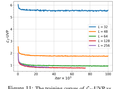Figure 11. The training curves of L2-UVP vs. iterations for OUR proposed method for the barycenter of Gaussian distributions depending on number of Langevin steps L

Mathematical & Logical Mechanism

The Master Equation

The absolute core mathematical engine powering this paper's approach to estimating entropic barycenters is the dual objective function that the algorithm seeks to maximize. This objective is derived from the weak dual formulation of the Entropic Optimal Transport (EOT) problem and is parameterized by neural networks. The specific equation optimized is given as:

$$ \mathcal{L}(\theta) \stackrel{\text{def}}{=} \sum_{k=1}^K \lambda_k \left\{ -\epsilon \mathbb{E}_{x_k \sim P_k} \left[ \log Z_{c_k}(f_{\theta,k}, x_k) \right] \right\} \quad (8) $$

where $Z_{c_k}(f_{\theta,k}, x_k)$ is the normalizing constant (or partition function) defined as:

$$ Z_{c_k}(f_{\theta,k}, x_k) \stackrel{\text{def}}{=} \int_{\mathcal{Y}} \exp\left(\frac{f_{\theta,k}(y) - c_k(x_k, y)}{\epsilon}\right) dy \quad (21) $$

Term-by-Term Autopsy

Let's break down these equations piece by piece to understand their roles:

• $\mathcal{L}(\theta)$: This is the objective function that the algorithm aims to maximize. Its value reflects how well the current set of potential functions (parameterized by $\theta$) aligns with the dual formulation of the EOT barycenter problem. Maximizing this dual objective is equivalent to minimizing the primal EOT barycenter problem.
• $\theta$: This represents the collection of all learnable parameters of the neural networks $f_{\theta,k}$. These parameters are adjusted during the learning process to optimize the objective.
• $K$: This is the total number of source probability distributions $P_k$ that we want to average. For example, if we are averaging three image datasets, $K=3$.
• $\lambda_k$: These are predefined positive weights for each source distribution $P_k$, such that $\sum_{k=1}^K \lambda_k = 1$. They dictate the relative importance or contribution of each source distribution to the final barycenter. If all $\lambda_k$ are equal, it's a simple average; otherwise, it's a weighted average.
• $\sum_{k=1}^K$: This is a summation operator that aggregates the contributions from all $K$ source distributions. The author uses addition because the EOT barycenter problem is formulated as a sum of individual EOT discrepancies between each source distribution and the barycenter.
• $\epsilon$: This is the entropic regularization parameter, a positive scalar. It controls the "smoothness" or "randomness" of the transport plans. A larger $\epsilon$ leads to more diffuse, less "sharp" transport plans (and a smoother loss landscape), while a smaller $\epsilon$ makes the transport more deterministic, approaching classical Optimal Transport. It acts as a "temperature" parameter in statistical mechanics.
• $\mathbb{E}_{x_k \sim P_k}[\dots]$: This denotes the expectation over samples $x_k$ drawn from the $k$-th source probability distribution $P_k$. In practice, this expectation is approximated using Monte Carlo sampling by drawing a batch of samples from $P_k$.
• $P_k$: This is the $k$-th source probability distribution. These are the input distributions that the algorithm aims to average. In real-world scenarios, these are typically only accessible via empirical samples (datasets).
• $x_k$: This is a sample (data point) drawn from the $k$-th source distribution $P_k$.
• $\log$: This is the natural logarithm function. It's used here because the weak entropic c-transform, $f_k^{c_k}(x_k)$, is defined as $-\epsilon \log Z_{c_k}(f_k, x_k)$. This transformation is crucial for converting the integral into a more manageable form for optimization and for relating it to energy-based models.
• $Z_{c_k}(f_{\theta,k}, x_k)$: This is the normalizing constant or partition function for the conditional probability distribution $\mu_{x_k}^{f_{\theta,k}}(y)$. It ensures that the conditional distribution integrates to 1. Its value depends on the potential function $f_{\theta,k}$ and the cost $c_k$ for a given $x_k$.
• $\int_{\mathcal{Y}} \dots dy$: This is an integral over the target space $\mathcal{Y}$. It sums up the "energy" contributions across all possible target points $y$ to compute the normalizing constant. The author uses an integral because the problem is set in a continuous domain of probability distributions.
• $\exp(\dots)$: This is the exponential function. It transforms the "energy" term $(f_{\theta,k}(y) - c_k(x_k, y))/\epsilon$ into a non-negative value that can be interpreted as an unnormalized probability density. This is a standard component in statistical mechanics and energy-based models.
• $f_{\theta,k}(y)$: This is the potential function for the $k$-th distribution, evaluated at a target point $y$. These functions are parameterised by neural networks $f_{\theta,k}$ and are the primary learnable components of the model. They represent the "value" or "utility" of a target point $y$ from the perspective of the $k$-th source.
• $c_k(x_k, y)$: This is the cost function for transporting mass from a source point $x_k$ to a target point $y$. It quantifies the dissimilarity or "cost" of moving between $x_k$ and $y$. The paper highlights its ability to handle general (even non-Euclidean) cost functions.
• $\frac{f_{\theta,k}(y) - c_k(x_k, y)}{\epsilon}$: This term represents the scaled "energy" or "log-probability" of transporting from $x_k$ to $y$, modulated by the potential $f_{\theta,k}$ and the regularization $\epsilon$. The potential $f_{\theta,k}(y)$ can be thought of as a "reward" for landing at $y$, while $c_k(x_k, y)$ is a "penalty" for the transport. The division by $\epsilon$ scales this energy, making the distribution sharper for small $\epsilon$ and flatter for large $\epsilon$.
• The subtraction $f_{\theta,k}(y) - c_k(x_k, y)$ within the exponent is a natural way to combine the potential and cost, as it reflects the net "attractiveness" of a target point $y$ for a given $x_k$.

Step-by-Step Flow

Imagine a single abstract data point, say $x_1$, from the first source distribution $P_1$, making its way through this mathematical engine during a training iteration.

1. Data Point Entry: A sample $x_1$ is drawn from the first source distribution $P_1$. This $x_1$ is a concrete instance from the dataset.
2. Potential Evaluation: For this $x_1$, and for a range of possible target points $y$ in the target space $\mathcal{Y}$, the neural network $f_{\theta,1}$ computes its potential $f_{\theta,1}(y)$. Simultaneously, the cost function $c_1(x_1, y)$ is evaluated, quantifying the "effort" to move from $x_1$ to each $y$.
3. Energy Calculation: These values are combined: $f_{\theta,1}(y) - c_1(x_1, y)$. This difference represents the "net utility" of transporting from $x_1$ to $y$. This utility is then scaled by the regularization parameter $\epsilon$, yielding $\frac{f_{\theta,1}(y) - c_1(x_1, y)}{\epsilon}$.
4. Unnormalized Probability: The scaled utility is exponentiated: $\exp\left(\frac{f_{\theta,1}(y) - c_1(x_1, y)}{\epsilon}\right)$. This gives an unnormalized measure of how "likely" it is to transport from $x_1$ to $y$.
5. Normalization (Partition Function): To make this a proper conditional probability distribution over $y$ (denoted $\mu_{x_1}^{f_{\theta,1}}(y)$), we need to normalize it. This is done by integrating the unnormalized probabilities over the entire target space $\mathcal{Y}$ to get $Z_{c_1}(f_{\theta,1}, x_1)$. This integral is often computationally intractable, so its gradient is estimated using techniques like MCMC.
6. Log-Likelihood Contribution: The natural logarithm of this normalizing constant, $\log Z_{c_1}(f_{\theta,1}, x_1)$, is then taken. This term, when multiplied by $-\epsilon$, effectively becomes the weak entropic c-transform $f_1^{c_1}(x_1)$.
7. Weighted Summation: This process (steps 2-6) is repeated for other samples from $P_1$ (to approximate the expectation $\mathbb{E}_{x_1 \sim P_1}[\dots]$) and for samples from all other source distributions $P_k$. Each distribution's contribution is then weighted by its $\lambda_k$ coefficient and summed up to form the total objective $\mathcal{L}(\theta)$.
8. Gradient Computation: The gradient of $\mathcal{L}(\theta)$ with respect to the neural network parameters $\theta$ is computed. This gradient indicates the direction in parameter space that would increase the objective function. As direct computation of $Z_{c_k}$ is hard, the gradient of $\log Z_{c_k}$ is approximated by sampling $y$ from the conditional distribution $\mu_{x_k}^{f_{\theta,k}}(y)$ using an MCMC procedure.
9. Parameter Update: Finally, the parameters $\theta$ of the neural networks $f_{\theta,k}$ are updated using an optimization algorithm (like stochastic gradient ascent) in the direction indicated by the computed gradient. This iterative update helps the model to gradualy adjust its potential functions to better satisfy the EOT barycenter conditions.

Optimization Dynamics

The mechanism learns by iteratively maximizing the dual objective function $\mathcal{L}(\theta)$ through stochastic gradient ascent. Here's how the learning, updating, and convergence unfold:

1. Neural Network Parameterization: The key insight is to represent the unknown potential functions $f_k$ as neural networks, $f_{\theta,k}$, where $\theta$ are the weights and biases of these networks. This allows for flexible, high-dimensional function approximation.
2. Congruence Condition Handling: The dual formulation (6) includes a crucial constraint: $\sum_{k=1}^K \lambda_k f_k = 0$. The authors ingeniously handle this by parameterizing $f_{\theta,k}$ as $g_{\theta,k} - \sum_{j=1}^K \lambda_j g_{\theta,j}$, where $g_{\theta,k}$ are individual neural networks. This specific construction automatically ensures that the sum of the weighted potentials is zero, eliminating the need for explicit constraint optimization.
3. Gradient Ascent: Since the objective function is a dual formulation, the goal is to maximize $\mathcal{L}(\theta)$. This is achieved using gradient ascent. The gradient $\frac{\partial}{\partial \theta} \mathcal{L}(\theta)$ is computed, and the parameters $\theta$ are updated in the direction of this gradient.
4. Gradient Estimation via MCMC: The most challenging part is computing the expectation $\mathbb{E}_{y \sim \mu_{x_k}^{f_{\theta,k}}} \left[ \frac{\partial}{\partial \theta} f_{\theta,k}(y) \right]$ within the gradient formula (Equation 9). The conditional distribution $\mu_{x_k}^{f_{\theta,k}}(y)$ has an unnormalized log-density given by $\frac{f_{\theta,k}(y) - c_k(x_k, y)}{\epsilon}$. To sample from this distribution, the paper employs a Markov Chain Monte Carlo (MCMC) procedure, specifically the Unadjusted Langevin Algorithm (ULA).
   • ULA Steps: For each $x_k$ sampled from $P_k$, ULA generates a sequence of samples $y_t$ that eventually approximate samples from $\mu_{x_k}^{f_{\theta,k}}$. The update rule for ULA is:
     $$y_{t+1}^{(1)} = y_t^{(1)} + \frac{\eta}{2\epsilon} \nabla_y (f_{\theta,k}(y) - c_k(x_k, y))|_{y=y_t^{(1)}} + \sqrt{\eta} \xi_t$$
     where $\eta$ is the step size, and $\xi_t$ is a random noise term drawn from a standard normal distribution. This process simulates a particle moving in an energy landscape defined by $f_{\theta,k}(y) - c_k(x_k, y)$, gradually converging to the target distribution.
5. Loss Landscape: The dual objective function is concave (as stated in Proposition A.1 (iii) for the weak c-transform, which extends to $\mathcal{L}(\theta)$). This concavity means that there are no local maxima that are not also global maxima, simplifying the optimization problem significantly compared to non-concave objectives. The entropy regularization parameter $\epsilon$ further smooths this landscape, making it easier for gradient-based methods to navigate and avoid getting stuck in spurious modes that might exist in the unregularized case.
6. Iterative Refinement: With each iteration, new samples $x_k$ are drawn, MCMC is run to generate $y$ samples, the gradient of $\mathcal{L}(\theta)$ is estimated, and $\theta$ is updated. This iterative process refines the neural network potentials $f_{\theta,k}$, causing them to converge towards the optimal potentials that define the EOT barycenter. The objective function is then maximised, and the barycenter is implicitly learned through these potentials.
7. Convergence: The paper provides theoretical guarantees (Theorem 4.2, 4.5, 4.6) regarding the quality of the recovered plans and the universal approximation capabilities of neural networks, suggesting that with sufficient data and network capacity, the learned potentials can accurately approximate the true EOT plans and thus the barycenter. However, practical convergence speed and quality are influenced by MCMC parameters (number of steps $L$, step size $\eta$) and batch size, as discussed in the experimental section.

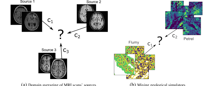Figure 6. A schematical presentation of potential applications of barycenter solvers

Results, Limitations & Conclusion

Experimental Design & Baselines

The authors meticulously designed a series of experiments to rigorously validate their proposed Energy-Guided Continuous Entropic Barycenter (EOT) solver across diverse scenarios, from low-dimensional toy problems to high-dimensional image manifolds. The core strategy for validation, especially when the ground truth barycenter is unknown, involved comparing the computed EOT barycenter (for a sufficiently small regularization parameter $\epsilon$) against the analytically derivable unregularized barycenter ($\epsilon=0$). This approach ruthlessly proved the efficacy of their mathematical claims by demonstrating qualitative and quantitative agreement or superior performance where applicable.

For 2D toy distributions, specifically the "twister" example, the experiment was architected with three comet-shaped 2D distributions ($P_1, P_2, P_3$) with uniform weights. Two distinct cost functions were tested: a non-Euclidean "twisted cost" $c_k(x_k, y) = ||u(x_k) - u(y)||^2$ and the standard Euclidean $l^2$ cost $c_k(x, y) = ||x - y||^2$, both with a regularization $\epsilon = 10^{-2}$. The "victims" or baselines here were the analytically derived true unregularized barycenter for the twisted cost (a centered Gaussian) and the $l^2$ barycenter estimated using the free_support_barycenter solver from the POT package [33]. This allowed for a direct comparison against known or well-established solutions. In the 3D sphere experiment, the solver estimated the barycenter of four von Mises distributions on a 3D sphere using a non-quadratic cost function $c_k(x_k, y) = \frac{1}{2} \arccos^2(x_k, y)$ and $\epsilon = 10^{-2}$. Here, the ground truth was unknown, so the evaluation was primarily qualitative, focusing on the reasonableness of the learned barycenter.

For image data, the experiments involved MNIST 0/1 digits and the Ave, celeba! dataset. For MNIST, the task was averaging distributions of 0/1 digits with equal weights in a $32 \times 32$ grayscale image space. The true unregularized $l^2$-barycenter for MNIST is a simple pixel-wise average, and the authors compared against existing solvers like SCWB [32] and WIN [55] which learn unregularized barycenters. Crucially, they introduced a manifold-constrained setup where the search space for the barycenter was restricted to a pre-trained StyleGAN [50] manifold, even "polluting" this manifold with irrelevant samples to test robustness. The cost function was modified to $c_{k,G}(x_k, z) = ||x_k - G(z)||^2$, with $\epsilon = 10^{-2}$. The Ave, celeba! dataset experiment involved averaging three degraded subsets of faces, where the true unregularized $l^2$ barycenter is the distribution of Celeba faces itself. This was also evaluated in the manifold-constrained setting with $\epsilon = 10^{-4}$, against SCWB [32] and WIN [55].

Finally, for Gaussian distributions, the authors conducted a quantitative evaluation using three Gaussian distributions in varying dimensions ($D = 2, 4, 8, 16, 64$) with weights $(\frac{1}{4}, \frac{1}{2}, \frac{1}{4})$ and regularization $\epsilon = 0.01, 1$. The ground truth unregularized barycenter $Q^*$ was estimated via an iterative procedure from the WIN repository, and the WIN solver [55] itself served as a baseline. The primary metric was the $L_2$-UVP (unexplained variance percentage) of the barycentric projections. Ablation studies were also performed to understand the impact of batch size and the number of Langevin steps. A single-cell experiment was also conducted, focusing on interpolating cell populations over time, with dimensions $D = 50, 100, 1000$. Here, the metric was MMD (Maximum Mean Discrepancy), and baselines included LightSB-M [2], SFM-sink [3], and EGNOT [1].

What the Evidence Proves

The experimental evidence definitively proves that the proposed Energy-Guided Continuous Entropic Barycenter (EOT) solver effectively approximates continuous EOT barycenters for general cost functions, overcoming limitations of prior methods.

The 3D sphere experiment (Figure 1) provides qualitative evidence that the approach is applicable to non-standard, non-quadratic experimental setups, producing reasonable barycenters even when the ground truth is unknown. This demonstrates the flexibility and robustness of the method beyond simple Euclidean spaces.

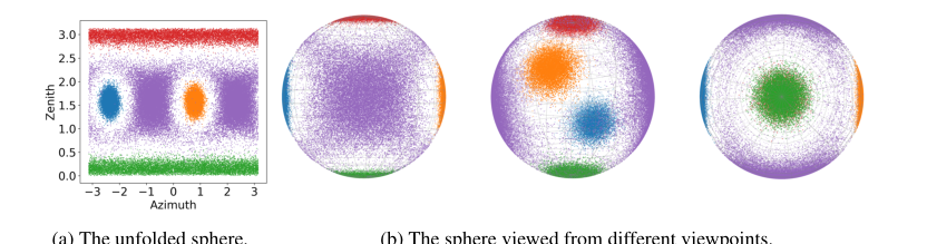Figure 1. Entropic barycenter Q∗(5) of N = 4 von Mises distributions Pn on the sphere (see M5.1) estimated with our barycenter solver (Algorithm 1). The used transport costs are ck(xk, y) = 1

For the 2D twister example, the qualitative results (Figure 12) show undeniable evidence that our solver, with $\epsilon = 10^{-2}$, accurately recovers the true unregularized barycenter for the non-Euclidean twisted cost. The computed barycenter (Fig. 12b) visually aligns perfectly with the analytically derived Gaussian ground truth (Fig. 12a). This is a strong validation of the core mechanism's ability to handle complex, non-Euclidean costs. For the $l^2$ cost, our EOT barycenter (Fig. 12d) also aligns well with the true $l^2$ barycenter (Fig. 12c), further confirming its general applicability. The distinct structures of the learned conditional plans for twisted vs. $l^2$ costs highlight the method's sensitivity to the underlying geometry defined by the cost function.

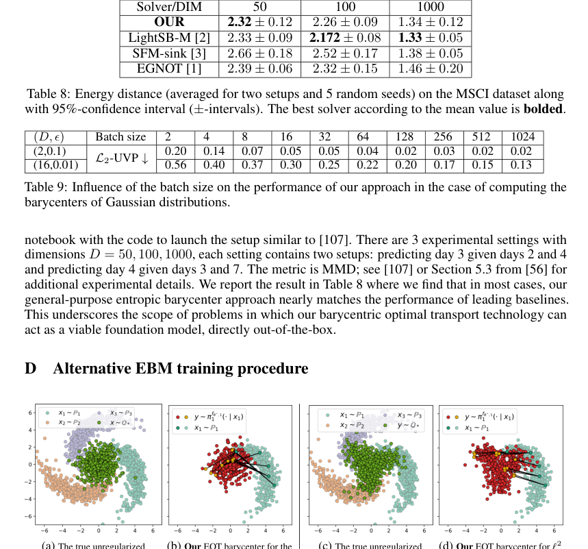Figure 12. 2D twister example. Trained with importance sampling: The true barycenter of 3 comets vs. the one computed by our solver with ϵ = 10−2. Two costs ck are considered: the twisted cost (12a, 12b) and ℓ2 (12c, 12d). We employ the simulation-free importance sampling procedure for training

In the MNIST 0/1 experiments, the "blurring bias" and noise observed in the data-space EOT barycenter (Figure 5, "OURS (Data Space)") are consistent with the nature of entropy-regularized OT and MCMC sampling. However, the manifold-constrained setup (Figure 5, "OURS (Manifold Constrained)") definitively proves the power of the proposed technique. By restricting the search to a StyleGAN manifold, the solver produces clean, interpretable barycenters, effectively ignoring "polluted" samples from the manifold. This is a crucial piece of evidence that the manifold constraint successfully alleviates the noise problem inherent in direct data-space EOT barycenter estimation.

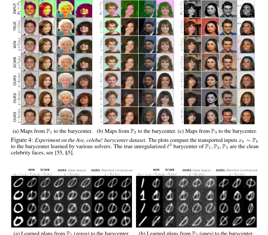Figure 5. Qualitative comparison of barycenters of MNIST 0/1 digit classes computed with barycenter solvers in the image space w.r.t. the pixel-wise ℓ2. Solvers SCWB and WIN only learn the unregularized barycenter (ϵ = 0) directly in the data space. In turn, our solver learns the EOT barycenter in data space as well as it can learn EOT barycenter restricted to the StyleGAN manifold (ϵ = 10−2)

The Ave, celeba! dataset evaluation provides compelling quantitative evidence. Our solver achieved significantly lower FID scores (Table 2) compared to the baseline models SCWB [32] and WIN [55]. For instance, our method's FID for $k=1$ was 8.4 (with a standard deviation of 0.3), dramatically outperforming SCWB's 56.7 and WIN's 49.3. This substantial improvement, particularly in the manifold-constrained setting, is definitive proof that the core mechanism, when combined with generative models, yields superior perceptual quality and more accurate barycenter estimation for complex image distributions. The qualitative results (Figure 4) also show "qualitatively good" transported images, despite occasional content preservation failures attributed to MCMC.

For Gaussian distributions, the quantitative $L_2$-UVP metric (Table 7) provides hard evidence of the solver's accuracy. For small $\epsilon = 0.01$ and dimensions up to $D=16$, our algorithm yielded $L_2$-UVP scores that were even better than the WIN solver, which is specifically designed for the unregularized case. For example, at $D=2$, our $L_2$-UVP was 0.02 compared to WIN's 0.03. This demonstrates that for appropriate regularization, our EOT solver can achieve state-of-the-art accuracy, even surpassing methods tailored for the unregularized setting. The ablation studies on batch size (Table 9) and Langevin steps (Figure 11) further confirm that the method's performance is sensitive to these parameters, with larger batch sizes and sufficient Langevin steps leading to improved quality, as expected from MCMC-based approaches.

Finally, the single-cell experiment (Table 8) shows that our general-purpose entropic barycenter approach nearly matches the performance of leading baselines (e.g., 2.32 for OURS vs. 2.33 for LightSB-M at $D=50$) across various dimensions and setups. This suggests its potential as a robust, out-of-the-box foundation model for problems like population interpolation.

Limitations & Future Directions

While the proposed Energy-Guided Continuous Entropic Barycenter solver demonstrates significant advancements, it is important to acknowledge its inherent limitations and to consider promising avenues for future research.

One of the primary methodological limitations stems from the reliance on Markov Chain Monte Carlo (MCMC) procedures during both training and inference. The basic Unadjusted Langevin Algorithm (ULA) used may suffer from poor convergence to the desired distribution $\mu^\ddagger$, especially in complex energy landscapes. MCMC sampling is also inherently time-consuming, which impacts the scalability of the method, particularly for larger batch sizes or higher-dimensional problems, as noted in the computational complexity analysis (Table 3, Appendix C). Future work should definitely explore more efficient sampling procedures, drawing inspiration from advanced MCMC techniques such as those involving replay buffers [46], auxiliary variables [43], or neural transport [47, 71, 99, 108, 66, 26]. This could significantly reduce computational burden and improve convergence stability.

Another theoretical limitation is that the current analysis of generalization bounds and universal approximation guarantees (§4.3) does not account for optimization errors arising from the gradient descent process and the MCMC sampling itself. This is a complex area of machine learning theory, distinct from the scope of this paper, but it represents a crucial direction for deeper theoretical understanding. Future research could aim to bridge this gap by developing a more comprehensive theoretical framework that integrates these practical optimization challenges.

From a problem setup perspective, the use of entropy regularization in image data space can lead to "blurring bias" and noisy barycenter images, as observed in the MNIST 0/1 data-space experiment (Figure 5). While the manifold-constrained approach effectively mitigates this by leveraging pre-trained generative models like StyleGAN, it introduces a dependency on the quality and suitability of these external models. The question then arises: how can we ensure the chosen manifold is truly representative of the underlying data structure, and how robust is the method to "polluted" or imperfect manifolds? Future work could investigate adaptive manifold learning techniques or methods for jointly learning the manifold and the barycenter, rather than relying on a fixed, pre-trained generative model.

A significant forward-looking discussion topic revolves around extending the energy-guided methodology to doubly-regularized EOT barycenters where the regularization parameters $\lambda$ and $\tau$ are not necessarily equal to $\epsilon$ (Appendix B.3). The current solver is tailored for the Schrödinger barycenter case ($\lambda = \tau = \epsilon$), where the entropy term $H(Q)$ disappears from the objective. Incorporating a non-zero $H(Q)$ term would require a separate, non-trivial computation of the entropy of the second marginals $\pi_k(y)$, which is currently infeasible from raw MCMC samples. Developing novel techniques to estimate or approximate this entropy term, or reformulating the dual objective to avoid its direct computation, would unlock a broader class of EOT barycenter problems.

Another critical area for future development lies in the design of appropriate cost functions and data manifolds for real-world applications, particularly in fields like medicine (domain shift problems) and geology (mixing simulators). The paper highlights that applying barycenters effectively in these domains requires domain-specific knowledge to define meaningful cost functions $c_k$ and to select or construct suitable data manifolds $M$. This suggests a need for interdisciplinary collaboration, bringing together machine learning experts with domain specialists to co-develop task-specific solutions. For instance, in medical imaging, exploring how to parameterize medical data manifolds using emerging large generative models (e.g., DALL-E [85], StableDiffusion [87]) could open new avenues for analysis.

The alternative Importance Sampling (IS) training procedure (Appendix D) shows promise for faster convergence but introduces its own challenge: the need for accurate selection of the proposal distribution $q$ to reduce estimator variance. This is often difficult in real-world scenarios. Future research could focus on developing adaptive or learned proposal distributions for IS, potentially combining it with MCMC or other techniques to create more robust and efficient training algorithms for EOT barycenters.

Finally, the scalability and computational efficiency remain key challenges. While the current method works for large-scale setups, the inference time, especially due to MCMC, can be substantial. Exploring hardware-accelerated MCMC, distributed computing strategies, or approximations that reduce the number of Langevin steps without significant quality degradation (as hinted by the ablation studies) would be valuable. The goal should be to make these continuous barycenter solvers more accessible and practical for industrial and socially-important problems, truly leveraging their potential as "foundation models" for optimal transport tasks.

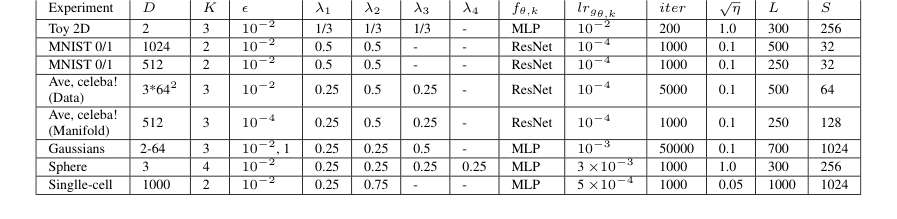Table 4. Hyperparameters that we use in the experiments with our Algorithm 1