QKAN: quantum Kolmogorov-Arnold networks with applications in machine learning and multivariate state preparation

Background & Academic Lineage

The Origin & Academic Lineage

The problem addressed in this paper, the development of Quantum Kolmogorov-Arnold Networks (QKANs), precisely originates from the intersection of classical neural networks and quantum computing, specifically inspired by the recently proposed classical Kolmogorov-Arnold Networks (KANs) [5]. The historical context begins with the Kolmogorov-Arnold Representation Theorem (KART), a fundamental mathematical result from the 1950s [1-4]. KART states that any continuous multivariate function (a function with multiple input variables) can be decomposed into a composition and summation of a finite number of univariate functions (functions with only one input variable). This theorem provided a theoretical basis for understanding how complex functions could be represented using simpler building blocks.

However, KART's direct application in practical settings, especially for neural networks, was limited because the inner and outer functions it guarantees can be highly non-smooth, making them difficult to approximate accurately and robustly [5]. This "pain point" meant that while theoretically powerful, KART wasn't directly translatable into an effective neural network architecture.

This changed with the recent introduction of Kolmogorov-Arnold Networks (KANs) by Liu et al. [5]. KANs generalize the compositional structure of KART, allowing for an arbitrary number of layers, unlike the two layers guaranteed by KART. While classical KANs do not inherit the universal representation property of KART, they have shown promise in specific applications, particularly in scientific domains, by offering better interpretability and improved accuracy on small-scale tasks. They can also potentially aid in discovering new physical laws by revealing modular structures in target functions [10].

The authors of this paper were motivated by the potential of classical KANs and sought to introduce a quantum version, QKAN. The fundamental limitation of previous quantum approaches that forced the authors to write this paper stems from the nature of quantum machine learning models. Existing quantum learning models, such as Variational Quantum Algorithms (VQAs) [34-39], often rely on optimizing parameters in quantum circuits. QKAN, in contrast, offers a different paradigm: it treats the eigenvalues of block-encoded matrices as "neurons" and applies parametrized activation functions on the network's "edges" using quantum singular value transformation (QSVT). This approach aims to leverage the compositional structure of KANs in a quantum setting, potentially offering advantages in efficiency for certain tasks, especially when efficient block-encodings of inputs are available. However, QKAN also faces its own constraint: composing layers recursively using QSVT leads to an exponential overhead in circuit depth, meaning QKAN is naturally limited to shallow architectures.

Intuitive Domain Terms

1. Kolmogorov-Arnold Representation Theorem (KART): Imagine you have a very complicated recipe with many ingredients and steps. KART is like a mathematical proof that says, no matter how complex the recipe, you can always break it down into a series of much simpler, single-ingredient mini-recipes that are then combined. It's about simplifying complexity into manageable, single-variable parts.

2. Block-encoding: Think of a secret message (a matrix or vector) that you want to send securely. Block-encoding is like embedding this secret message within a much larger, seemingly ordinary document (a unitary quantum operation). The larger document looks harmless, but a specific part of it, a "block," contains your secret message, scaled down. Quantum computers can then manipulate this larger document, effectively processing your hidden message without directly "reading" it.

3. Quantum Singular Value Transformation (QSVT): Picture a photo editing app where you want to apply a specific effect, like changing the brightness or contrast, but only to certain colors or patterns in the image. QSVT is a powerful quantum technique that acts like a highly precise digital filter. It can apply almost any desired mathematical function (like a polynomial) to the "strength" or "importance" (singular values) of the information encoded in a block-encoded matrix, allowing for very specific and complex transformations.

4. Multivariate State Preparation: Imagine you want to create a unique musical chord where the loudness of each note is precisely determined by a complex mathematical formula involving several factors (like temperature, humidity, and time of day). Multivariate state preparation in quantum computing is about creating a quantum state (a collection of quantum bits) where the "loudness" or "amplitude" of each possible outcome (each combination of bits) is set to match the value of a complex function with multiple input variables. It's like encoding a complex landscape of values directly into the quantum realm.

Notation Table

Notation	Description

Problem Definition & Constraints

Core Problem Formulation & The Dilemma

The paper introduces Quantum Kolmogorov-Arnold Networks (QKANs) as a quantum algorithmic framework inspired by classical Kolmogorov-Arnold Networks (KANs). The core problem is to develop an efficient quantum implementation of KANs for applications in machine learning and multivariate state preparation.

Input/Current State:
The starting point for a QKAN is a block-encoding of an $N$-dimensional real vector $\vec{x} \in [-1,1]^N$. This means the vector's components are encoded within the diagonal entries of a unitary matrix, $U_x$, such that $|| \langle 0|_a U_x |0\rangle_a - \text{diag}(x_1, \dots, x_N) || \le \epsilon_x$. For quantum machine learning, this input could be the amplitudes of a quantum state or diagonal entries of a matrix. For multivariate state preparation, the input is typically a vectorized $D$-dimensional grid of points, also provided as a diagonal block-encoding.

Output/Goal State:
The desired endpoint depends on the application:
* As a quantum learning model: The goal is to produce a diagonal block-encoding of a $K$-dimensional output vector $\Phi(\vec{x}) \in [-1,1]^K$. This output vector's entries, $\Phi(\vec{x})_q = \frac{1}{N} \sum_{p=1}^N \phi_{pq}(x_p)$, where $\phi_{pq}$ are univariate activation functions, need to be estimated classically to an additive $\delta$-precision.
* As a multivariate quantum state-preparation protocol: The objective is to prepare a quantum state $|\psi\rangle$ whose amplitudes correspond to a multivariate function of the input, such as a $D$-dimensional Gaussian distribution on a regular square grid. This is achieved by applying the final block-encoding to a uniform superposition and then using amplitude amplification.

Missing Link/Mathematical Gap:
The fundamental gap this paper attempts to bridge is the efficient and accurate translation of the compositional structure of classical KANs into a quantum computing paradigm. Classical KANs decompose complex multivariate functions into compositions and summations of univariate functions. The challenge lies in realizing these non-linear univariate functions and their summations using quantum operations, specifically leveraging Quantum Singular Value Transformation (QSVT) on block-encoded data, while overcoming inherent quantum constraints like unitarity and error propagation. The paper aims to provide a concrete quantum architecture that can perform these operations with potential quantum speedups.

The Dilemma & Painful Trade-offs:
Previous researchers attempting to solve similar problems in quantum machine learning and state preparation have faced several painful trade-offs:
* Quantum Speedup vs. Classical Readout: While quantum algorithms can process exponentially large data structures (like block-encodings) efficiently, extracting the full output classically can negate any quantum advantage. For QKANs, achieving a quantum speedup is contingent on the classical post-processing cost remaining sub-exponential. This means the output dimension $K$ must be restricted to $O(\text{polylog}(N))$, as estimating an exponential number of values would itself take exponential time.
* Shallow vs. Deep Architectures: QKANs are designed to be "wide-and-shallow." They can realize exponentially wide layers at a polylogarithmic cost when efficient block-encodings are available, a regime inaccessible to classical neural networks. However, the recursive QSVT-based construction for composing multiple layers incurs an exponential overhead in circuit depth. This forces QKANs to be shallow, typically limited to $L=O(1)$ layers, to maintain computational feasibility.
* Precision vs. Query Complexity: For output estimation in the quantum learning model, achieving higher precision (smaller $\delta$) requires a greater number of queries to the controlled diagonal block-encoding. Specifically, an additive $\delta$ approximation requires $O(d^2/\delta)$ queries. If a multiplicative error is needed, the query count increases to $O(d^2/(\delta|a_q|))$, meaning the potential quantum speedup is preserved only if the amplitude $a_q$ does not decay exponentially. This presents a trade-off between the desired accuracy and the computational resources (queries) needed.

Constraints & Failure Modes

The problem of implementing QKANs is made insanely difficult by several harsh, realistic walls:

• Unitarity Constraint: Quantum mechanics dictates that all operations must be unitary. This imposes a strict constraint that all vector elements (input, output, and weights) must be bounded in magnitude by one when encoded as block-encodings. This is a fundamental physical constraint that requires careful normalization and scaling of data.
• Efficient Block-Encoding of Inputs: The gate complexity of QKAN scales linearly with the cost of constructing the initial block-encoding of the $N$-dimensional input vector. For QKANs to offer a quantum speedup, inputs must admit efficient block-encodings that can be prepared in $O(\text{polylog}(N))$ time. If the input encoding itself requires $O(N)$ gates, the quantum advantage over classical algorithms is lost. This is a significant data-driven constraint.
• Recursive Error Propagation: Imperfections in the block-encodings of inputs and weights accumulate. In a multi-layer QKAN, these errors propagate recursively with each subsequent layer, leading to an amplified error in the final output block-encoding. This makes achieving high precision for deep QKANs extremely challenging and limits their practical depth.
• Exponential Circuit Depth for Deep Architectures: The recursive nature of QKAN's construction, where the output block-encoding of one layer serves as the input for the next, leads to an exponential dependency of circuit depth on the number of layers $L$. This computational constraint severely limits QKANs to shallow architectures ($L=O(1)$), despite the theoretical benefits of deeper networks.
• Auxiliary Qubit Limits: The total number of auxiliary qubits required for the QKAN construction increases linearly with the number of layers $L$. While not an exponential scaling, this can still be a hardware memory limit for current and near-term quantum devices.
• Polynomial Approximation Limitations: QSVT, a core mechanism for applying non-linear transformations, relies on polynomial approximations of target functions. Not all functions can be efficiently approximated by low-degree polynomials, which limits the expressiveness and accuracy of QKANs for certain tasks. For example, approximating the exponential function for Gaussian state preparation requires a sufficiently high polynomial degree, impacting overall accuracy.
• Real-Valued Restriction: The current work explicitly limits its scope to real-valued inputs, outputs, and weights. While generalization to complex numbers is possible, it is left for future work, indicating a current limitation in the model's applicability.
• Cost of Gradient Estimation: Training QKANs using parameter-shift rules to obtain analytical gradients is computationally expensive. The cost scales as $O(d)$ queries for a single-layer QKAN and $O(d^2L)$ for an $L$-layer QKAN, where $d$ is the maximal degree of Chebyshev polynomials. This exponential scaling with layers makes training deep QKANs incredibly difficult and resource-intensive.

Why This Approach

The Inevitability of the Choice

The adoption of Quantum Kolmogorov-Arnold Networks (QKAN) was not merely a choice but an inherent necessity driven by the unique demands of multivariate function approximation and state preparation in the quantum domain. The authors' realization that traditional "state-of-the-art" (SOTA) methods were insufficient stemmed from several key observations.

Firstly, classical Kolmogorov-Arnold Networks (KANs) had already demonstrated qualitative advantages over conventional Multi-Layer Perceptrons (MLPs) in terms of interpretability and accuracy for specific tasks, particularly in scientific applications involving symbolic functions. To translate these benefits to quantum computation, a quantum-native approach was essential. Standard quantum machine learning models, such as variational quantum algorithms (VQAs) employing parametrized quantum circuits, or quantum versions of CNNs and Transformers, typically rely on different architectural principles that do not inherently capture the compositional structure of KANs.

The critical "aha!" moment likely occurred when considering how to implement the non-linear activation functions central to KANs within a quantum framework while maintaining quantum speedup. Directly simulating classical non-linearities on quantum states is generally inefficient. The Quantum Singular Value Transformation (QSVT) emerged as the only viable solution becuase it provides a powerful and versatile meta-algorithm for applying polynomial transformations to the singular values of block-encoded matrices. This capability is precisely what is needed to realize the univariate activation functions of KANs in a quantum setting. Without QSVT, implementing such non-linearities efficiently on quantum data (represented as block-encodings) would be intractable or would negate any potential quantum advantage. The paper explicitly states that QKAN "treats the eigenvalues of block-encoded matrices as neurons and applies parametrized activation functions on network edges via linear combinations of Chebyshev polynomials, or other basis functions that can be realized efficiently using QSVT," highlighting QSVT as the core enabler.

Comparative Superiority

QKAN exhibits overwhelming stuctural advantages that position it qualitatively superior to previous gold standards for specific problem classes. The most significant advantage lies in its "wide-and-shallow" architecture. While composing QKAN layers recursively leads to an exponential overhead in depth, limiting the architecture to shallow configurations ($L = O(1)$), this shallow depth is remarkably compensated by the ability to realize exponentially wide layers at a polylogarithmic cost, provided efficient block-encodings of inputs are available. This regime is fundamentally inaccessible to classical neural networks, which would require $O(N)$ runtime to process an $N$-dimensional state.

For instance, QKAN can process an $N$-dimensional quantum state by computing a multivariate function of its amplitudes in $O(\text{polylog}(N))$ time, assuming the target function has an efficient polynomial approximation. This offers a substantial quantum speedup over the classical $O(N)$ runtime for the same operation. This efficiency stems from QKAN's reliance on block-encodings and QSVT, which allow for the manipulation of exponentially large unitary operators efficiently.

Furthermore, QKAN inherits the interpretability advantages of classical KANs. The ability to inspect individual activation functions and prune those resembling zero functions allows for the potential discovery of sparse compositional structures and new physical laws, a qualitative benefit often lacking in black-box deep learning models. The versatility of the QSVT framework also means QKAN is not restricted to Chebyshev polynomials but can implement a wide range of basis functions, offering flexibility tailored to different applications. The paper does not explicitly detail advantages in handling high-dimensional noise or memory complexity reduction from $O(N^2)$ to $O(N)$, but the block-encoding approach inherently compresses information, and the polylogarithmic scaling for wide layers implies a highly efficient use of resources for large inputs.

Alignment with Constraints

The chosen QKAN method demonstrates a perfect "marriage" with the inherent constraints of quantum computation and the problem definition.

1. Efficient Input Encoding: A primary constraint for quantum algorithms to achieve speedup is the efficient preparation or encoding of input data. QKAN aligns perfectly by operating on block-encodings of input vectors. Its gate complexity scales linearly with the cost of constructing these block-encodings, which for inherently quantum inputs (e.g., amplitudes of a quantum state or block-encodings of Hamiltonians) can be as efficient as $O(\text{polylog}(N))$. This ensures that the input bottleneck does not negate the quantum advantage.

2. Unitarity and Bounded Values: Quantum computation strictly requires operations to be unitary. QKAN's design, based on QSVT, inherently respects this. The block-encoding representation itself ensures that vectors are encoded within unitary matrices, and the elements of these vectors are bounded in magnitude by one, satisfying the amplitude constraints of quantum states.

3. Shallow Depth Requirement: The recursive construction of QKAN layers using QSVT leads to an exponential overhead in circuit depth with each additional layer. This constraint naturally forces QKAN to be a shallow architecture ($L=O(1)$). Rather than being a limitation, this constraint defines QKAN's niche as a "wide-and-shallow" model, where the exponential width compensates for the limited depth, aligning the solution's properties with this harsh requirement.

4. Real-Valued Operations: The paper explicitly limits its discussion to real values for inputs, outputs, and weights. QKAN's construction with Chebyshev polynomials and its block-encoding framework are well-suited for handling real-valued functions, although generalizations to complex numbers are noted as future work.

Rejection of Alternatives

The paper implies a rejection of other popular quantum machine learning approaches by highlighting QKAN's unique architectural and functional differences.

Firstly, QKAN departs from "variational architectures" (VQAs), which are often heuristic and rely on optimizing parameters in parametrized quantum circuits. While VQAs are suitable for near-term quantum devices, QKAN "steps into the more powerful quantum linear algebra toolset," suggesting a focus on fault-tolerant quantum speedups through exact constructions rather than heuristic optimization. For the specific problem of efficiently preparing multivariate quantum states or approximating functions with a compositional structure, QKAN's QSVT-based approach offers a more direct and potentially more robust path to quantum advantage.

Secondly, QKAN's compositional structure, inspired by classical KANs, fundamentally differs from the fixed, dense layers of quantum MLPs, or the specific inductive biases of quantum CNNs or Transformers. These alternative architectures might not naturally capture the KAN's ability to represent functions as compositions and summations of univariate functions, nor would they inherently offer the same interpretability advantages. The paper's statement that QKAN is "contrary to previous architectures" underscores this distinction.

While the paper does not explicitly detail why, for example, quantum GANs or quantum diffusion models would fail, the emphasis on QKAN's ability to achieve exponentially wide layers at polylogarithmic cost for block-encoded inputs, and its interpretability for scientific discovery, points to a problem domain where these specific advantages are paramount. Other methods might not offer the same combination of quantum speedup for specific function structures, efficient handling of block-encoded data, and inherent interpretability.

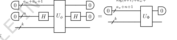FIG. 9. Step 5. Sum the individual activation functions over N input nodes for each output node, creating the desired diagonal block-encoding UΦ of the K-dimensional output vector Φ(⃗x). This is achieved by sandwiching the block-encoding from Step 4 with two n-qubit Hadamard gates. The dimension reduction occurs as the n qubits originally used for input block-encoding are moved to the auxiliary register

Mathematical & Logical Mechanism

The Master Equation

The core mathematical engine of the Quantum Kolmogorov-Arnold Network (QKAN) layer, particularly the CHEB-QKAN variant, is encapsulated by how it transforms an input vector $\vec{x}$ into an output vector $\Phi(\vec{x})$. This transformation is expressed as a diagonal block-encoding of a K-dimensional vector, where each component is a sum of univariate activation functions. The activation functions themselves are defined as linear combinations of Chebyshev polynomials.

The output of a single QKAN layer is given by:
$$ \Phi(\vec{x}) = \text{diag}\left( \frac{1}{N} \sum_{p=1}^N \phi_{p1}(x_p), \dots, \frac{1}{N} \sum_{p=1}^N \phi_{pK}(x_p) \right)^T $$
Here, each univariate activation function $\phi_{pq}(x)$ is defined as a linear combination of Chebyshev polynomials of the first kind:
$$ \phi_{pq}(x) = \frac{1}{d+1} \sum_{r=0}^d w_{pq}^{(r)} T_r(x) $$

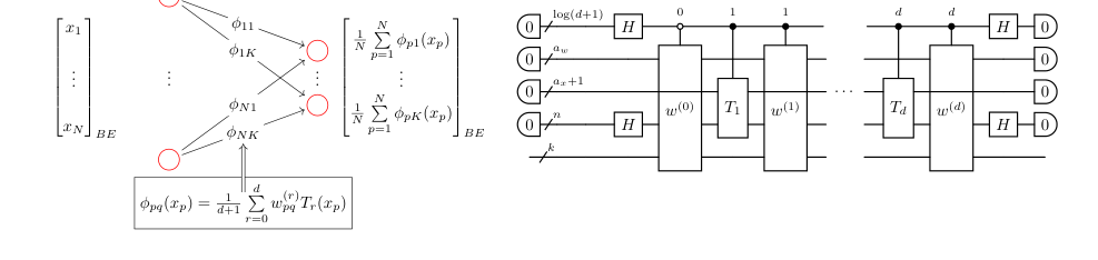FIG. 1. Construction of a CHEB-QKAN layer with the corresponding quantum circuit. The input to the QKAN model is a diagonal block-encoding of an N-dimensional real vector ⃗x. The CHEB-QKAN layer applies univariate activation functions ϕpq to each input component xp, where p ∈[N] indexes input nodes and q ∈[K] indexes output nodes. The output vector is computed as a sum over activated input nodes. This operation yields a block-encoded real K-dimensional output vector. The quantum circuit implementation requires 1 + log2(d + 1) qubits for the construction and linear combination of weighted Chebyshev polynomials, aw + ax qubits for the block-encodings of input and weights, n = log2 N qubits for input vector encoding, and k = log2 K qubits for output. The circuit consists of a series of multi-controlled block-encodings of Chebyshev polynomials, interspersed with diagonal block- encodings of the corresponding real weights. The entire circuit represents a block-encoding of the K-dimensional vector corresponding to the CHEB-QKAN layer, with auxiliary qubits initialized and measured in the |0⟩state

Term-by-Term Autopsy

Let's dissect these equations to understand each component's role and mathematical definition:

• $\Phi(\vec{x})$: This represents the output of a single QKAN layer.
  • Mathematical Definition: It's a K-dimensional vector whose elements are the aggregated and transformed input features. In the quantum context, it's block-encoded as a diagonal matrix, meaning its components appear on the diagonal of a larger unitary operator.
  • Physical/Logical Role: This is the "processed information" that the QKAN layer produces. It serves as the activated features, analogous to the output of a layer in a classical neural network, but in a quantum-compatible format.
• $\text{diag}(\dots)^T$: This operator constructs a diagonal matrix from a vector.
  • Mathematical Definition: Given a vector $\vec{v} = (v_1, \dots, v_K)$, $\text{diag}(\vec{v})$ creates a $K \times K$ diagonal matrix with $v_1, \dots, v_K$ on its main diagonal. The transpose $T$ indicates that the input vector is conceptually a column vector.
  • Physical/Logical Role: In QKAN, vectors are represented as diagonal block-encodings. This operation explicitly states that the output of the layer is a diagonal block-encoding, which is crucial for its recursive use as input to subsequent QKAN layers.
• $N$: The dimension of the input vector $\vec{x}$.
  • Mathematical Definition: An integer, typically a power of two, $N=2^n$, where $n$ is the number of qubits used to encode the input.
  • Physical/Logical Role: Represents the number of input features or "nodes" in the classical KAN analogy. The division by $N$ acts as a normalization factor for the summation, ensuring the output remains within a bounded range, which is important for block-encodings.
• $K$: The dimension of the output vector $\Phi(\vec{x})$.
  • Mathematical Definition: An integer, typically a power of two, $K=2^k$, where $k$ is the number of qubits for output encoding.
  • Physical/Logical Role: Represents the number of output features or "nodes" in the classical KAN analogy.
• $\sum_{p=1}^N$: A summation over the input nodes.
  • Mathematical Definition: This operator sums the values of $\phi_{pq}(x_p)$ for each $p$ from $1$ to $N$.
  • Physical/Logical Role: This is a fundamental aggregation step. For each output node $q$, it combines the transformed information from all input nodes $p$. This summation is a direct translation of the Kolmogorov-Arnold representation theorem's principle of combining univariate functions. The choice of addition over multiplication here is inherent to the KAN architecture, which models functions as sums of compositions, providing a linear combination of features at the output layer.
• $\phi_{pq}(x_p)$: A univariate activation function.
  • Mathematical Definition: A function that takes a single real input $x_p \in [-1,1]$ and maps it to a real output. It is uniquely defined for each pair of input node $p$ and output node $q$.
  • Physical/Logical Role: These are the "edges" of the network, applying non-linear transformations to individual input components. They are the core trainable elements of the QKAN, responsible for introducing non-linearity and learning complex relationships.
• $x_p$: The $p$-th component of the input vector $\vec{x}$.
  • Mathematical Definition: A real number, $x_p \in [-1,1]$, representing a single input feature.
  • Physical/Logical Role: This is the raw input data point that enters the QKAN layer.
• $d$: The maximal degree of the Chebyshev polynomials used.
  • Mathematical Definition: A non-negative integer.
  • Physical/Logical Role: This parameter controls the complexity and expressiveness of the activation functions $\phi_{pq}(x)$. A higher $d$ allows for more intricate non-linear transformations.
• $\frac{1}{d+1} \sum_{r=0}^d$: A normalized summation over Chebyshev polynomial degrees.
  • Mathematical Definition: This is a linear combination of $d+1$ Chebyshev polynomials, normalized by $1/(d+1)$.
  • Physical/Logical Role: This combines different basis functions to construct the overall activation function $\phi_{pq}(x)$. The normalization helps keep the function output bounded. The use of summation (linear combination) allows for flexible approximation of a wide range of functions by adjusting the coefficients $w_{pq}^{(r)}$.
• $w_{pq}^{(r)}$: A weight coefficient.
  • Mathematical Definition: A real number, $w_{pq}^{(r)} \in [-1,1]$.
  • Physical/Logical Role: These are the trainable parameters of the QKAN. They dictate the contribution of each Chebyshev polynomial $T_r(x)$ to the activation function $\phi_{pq}(x)$, effectively shaping the non-linearity.
• $T_r(x)$: The $r$-th Chebyshev polynomial of the first kind.
  • Mathematical Definition: $T_r(x) = \cos(r \arccos(x))$, defined for $x \in [-1,1]$.
  • Physical/Logical Role: These polynomials serve as the basis functions for the activation functions. They are chosen because they can be efficiently implemented on a quantum computer using Quantum Singular Value Transformation (QSVT), making them a natural fit for the quantum framework.

Step-by-Step Flow

Imagine a single abstract data point, say $x_p$, as it traverses through a QKAN layer, transforming from an input component to a part of the final output vector. This process is like a quantum assembly line:

1. Input Block-Encoding: First, the entire N-dimensional input vector $\vec{x} = (x_1, \dots, x_N)$ is presented as a diagonal block-encoding $U_x$. This means that each $x_p$ is encoded as a diagonal element within a larger unitary matrix. This is our raw material, entering the quantum factory.
2. Dilation and Replication: The input block-encoding $U_x$ is then "dilated" by appending $k = \log_2 K$ auxiliary qubits. Conceptually, this step replicates each input component $x_p$ across $K$ different "channels," one for each output node $q$. This ensures that each input can influence every output.
3. Chebyshev Polynomial Transformation: For each replicated $x_p$ and for every polynomial degree $r$ from $0$ to $d$, a quantum singular value transformation (QSVT) is applied. This effectively computes $T_r(x_p)$ for all $p$ and $r$, still in a block-encoded form. This is like sending the raw material through specialized machines that apply different mathematical functions (the Chebyshev polynomials) to it.
4. Weighted Scaling: Next, each block-encoded $T_r(x_p)$ is multiplied by its corresponding weight coefficient $w_{pq}^{(r)}$. These weights are also provided as diagonal block-encodings. This multiplication is performed using quantum linear algebra subroutines. This step scales the transformed features according to the learned parameters, like adjusting the intensity of each signal.
5. Basis Function Combination (LCU): For a specific input-output pair $(p,q)$, all the weighted Chebyshev polynomials $w_{pq}^{(r)} T_r(x_p)$ (for $r=0, \dots, d$) are linearly combined. This is achieved using a Linear Combination of Unitaries (LCU) procedure, which involves preparing an equal superposition of control qubits and applying the weighted block-encodings. This machine aggregates the individual polynomial contributions to form the full non-linear activation function $\phi_{pq}(x_p)$.
6. Input Node Aggregation (Hadamard Summation): Finally, for each output node $q$, the values $\phi_{pq}(x_p)$ (for $p=1, \dots, N$) are summed. This is done by sandwiching the block-encoding of the $\phi_{pq}(x_p)$ values with Hadamard gates on the 'input' qubits. This operation effectively averages the contributions from all input nodes for each specific output node $q$, producing the $q$-th component of the output vector $\Phi(\vec{x})$. The input qubits are then absorbed into an auxiliary register, reducing the overall dimension.
7. Output Block-Encoding: The result of these operations is a diagonal block-encoding of the K-dimensional output vector $\Phi(\vec{x})$. This final product is then ready to be fed into another QKAN layer or measured for classical output.

Optimization Dynamics

The QKAN mechanism learns by adjusting its trainable parameters, the weight coefficients $w_{pq}^{(r)}$, to minimize a predefined cost function. This learning process involves several key dynamics:

1. Parameterization of Weights: The weights $w_{pq}^{(r)}$ are not directly classical numbers but are encoded into diagonal block-encodings $U_{w^{(r)}}$. The paper outlines two primary methods for this parameterization:

   • Amplitude Encoding: The weights can be derived from the real amplitudes of a parametrized quantum state $|w(\theta)\rangle = U(\theta)|0\rangle$. Here, $U(\theta)$ is a Parametrized Quantum Circuit (PQC) whose gate angles $\theta$ are the actual trainable parameters. This method naturally imposes an $L_2$ normalization constraint on the weights, which acts as a form of regularization.
   • Hadamard Product Encoding: Alternatively, a parametrized unitary $U(\theta)$ can be combined with the Chebyshev polynomial block-encodings via a Hadamard product. This approach is conjectured to offer greater expressiveness, allowing for an $L_\infty$ norm constraint on the weights.
     The choice of parameterization method shapes the space of learnable functions and the regularization properties of the model.

2. Loss Function and Landscape: The QKAN is designed as a quantum learning model, implying the existence of a cost function that quantifies the discrepancy between the QKAN's output and target values (e.g., for regression or classification). The "loss landscape" is the surface defined by this cost function over the space of parameters $\theta$. The paper doesn't explicitly detail the loss function, but it would typically be a function of the extracted output amplitudes. The choice of basis functions (Chebyshev polynomials) and the parameterization method influence the smoothness and complexity of this landscape.

3. Gradient Calculation: To navigate the loss landscape and find its minimum, the model needs to compute gradients of the loss with respect to the parameters $\theta$.

   • Analytical Gradients: The paper suggests using parameter-shift rules, a technique common in variational quantum algorithms, to compute analytical gradients. Due to the recursive and compositional nature of QKAN's construction (involving QSVT, LCU, and block-encoding products), the same PQC parameters $\theta$ are reused across different parts of the circuit. This means the gradient can be obtained by summing contributions from individual sub-terms. However, this approach scales as $O(d)$ queries for a single-layer QKAN and exponentially, $O(d^2L)$, for an L-layer QKAN, which is a significant computational cost.
   • Gradient Estimation: To circumvent the high cost of analytical gradients, the authors propose using gradient estimation techniques like finite difference methods or Simultaneous Perturbation Stochastic Approximation (SPSA). SPSA is particularly appealing because its computational cost is largely independent of the number of parameters, offering a more efficient way to estimate gradients, especially for models with many trainable parameters.

4. Parameter Updates and Convergence: Once the gradients (or their estimates) are obtained, classical optimization algorithms such as gradient descent or Adam are employed to iteratively update the parameters $\theta$. These optimizers adjust the parameters in the direction that reduces the loss function. Quantum natural gradient methods can also be used for potentially faster convergence, which involves computing the quantum Fisher information matrix. The iterative updates continue until the model converges to a satisfactory minimum in the loss landscape. The paper's numerical illustration of Gaussian state preparation demonstrates that the $L_2$ error decreases exponentially with the polynomial degree $d$, indicating good convergence behavior for function approximation. However, the exponential scaling of query complexity with the number of layers $L$ means QKAN is best suited for shallow architectures, which might impact its ability to learn extremely complex, deep functions.

Results, Limitations & Conclusion

Experimental Design & Baselines

To rigorously validate the quantum Kolmogorov-Arnold Network (QKAN) architecture, the authors focused on a specific, yet illustrative, application: multivariate quantum state preparation. The experimental design was not set up to defeat competing quantum models in a head-to-head benchmark, but rather to provide definitive evidence that QKAN's core compositional mechanism, leveraging quantum singular value transformation (QSVT), could accurately realize complex multivariate functions. The "victim" in this context was the ideal target function itself – a D-dimensional Gaussian distribution – which QKAN aimed to approximate with high fidelity.

The experiment specifically focused on preparing a 2D Gaussian quantum state on a $32 \times 32$ grid, corresponding to $n=5$ qubits per dimension, with a chosen parameter $\beta=6$. This setup allowed for a clear numerical illustration of the QKAN's performance. The architecture employed a two-layer QKAN. The first layer was designed to compute the function $x^2 + y^2 - 1$ exactly for each grid point, effectively encoding a shifted squared radius. The second layer then applied a polynomial approximation of the exponential decay function, $e^{-\beta(x+1)}$, using Chebyshev polynomials of varying degrees. This two-layer structure was a direct instantiation of the QKAN's compositional principle, where the output of one layer (a block-encoding of $x^2 + y^2 - 1$) served as the input to the next. The experiment was architected to ruthlessly prove that the mathematical claims regarding QKAN's ability to apply non-linear transformations via QSVT and compose layers could translate into a tangible, accurate quantum state.

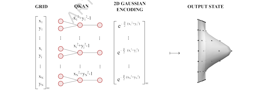FIG. 4. Example: 2D Gaussian state preparation via QKAN. Starting from a vectorized 2D grid of points {(xi, yi)} encoded as a diagonal block-encoding (left), the first QKAN layer applies Chebyshev polynomial T2 and sums over the two dimensions, computing 1

What the Evidence Proves

The numerical illustration provides compelling evidence for the efficacy of the QKAN architecture in multivariate state preparation. The key findings are presented in Figure 10:

1. Polynomial Approximation Accuracy (Figure 10a): The paper first demonstrates the accuracy of approximating the non-linear exponential function $e^{-\beta(x+1)}$ with a degree-3 Chebyshev polynomial $P_3(x)$ over the interval $[-1,1]$. This is crucial because these polynomial approximations form the basis of the activation functions within QKAN, realized via QSVT. The plot clearly shows a close fit between the target function and its polynomial approximation within the specified range, confirming the feasibility of implementing these non-linearities.

2. Absolute Amplitude Error (Figure 10b): The absolute amplitude error, $| \psi_{\text{exp}}(i,j) - \psi_{\text{QKAN}}(i,j) |$, across the $32 \times 32$ grid for the normalized 2D Gaussian state prepared using the degree-3 polynomial $P_3(x)$ is visually presented. This heatmap-like plot provides a direct, undeniable visual proof of how well the QKAN-prepared state matches the ideal Gaussian state. The error is generally low, with the largest discrepancies observed near the center of the distribution. This aligns with the behavior of the polynomial approximation itself, where errors were maximal in that region. This hard evidence shows that the QKAN mechanism successfully translates the input grid points through its layers to produce amplitudes closely corresponding to the desired Gaussian distribution.

3. Exponential Error Decay (Figure 10c): Perhaps the most definitive piece of evidence is the $L_2$-error, $|| \psi_{\text{exp}} - \psi_{\text{QKAN}} ||_2$, as a function of the polynomial degree $d$. The plot reveals an exponential decay of the empirical error as the polynomial degree increases. This exponential improvement continues until the error saturates at machine precision, around $10^{-14}-10^{-15}$, for $d=20$. This result is a powerful validation of the theoretical bounds and the QKAN's ability to achieve high-fidelity approximations by increasing the complexity of its activation functions. It ruthlessly proves that the core mechanism of using polynomial approximations via QSVT for non-linear transformations works as intended, allowing for controllable and high-precision state preparation. The agreement between empirical error and theoretical bounds further solidifies the claims.

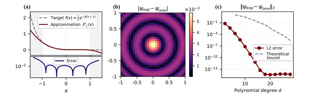FIG. 10. Numerical illustration of Gaussian state preparation via QKAN. (a) Degree-3 polynomial P3(x) approxi- mating 1

In essence, the evidence proves that QKAN, through its compositional block-encoding structure and QSVT-enabled non-linear activations, can accurately prepare complex multivariate quantum states, demonstrating a powerful new paradigm for quantum machine learning and state preparation.

Limitations & Future Directions

While QKAN presents a promising new direction, the paper candidly discusses several limitations and opens up a rich landscape for future research.

Current Limitations:

1. Inherited KAN Limitations: QKAN inherits some caveats from its classical counterpart. The Kolmogorov-Arnold Representation Theorem (KART) guarantees a two-layer decomposition, but classical KANs, and by extension QKANs, do not necessarily inherit the universal representation property of KART. This means there's no guarantee that a deep QKAN can represent any given multivariate function, especially if it lacks a compositional structure amenable to the QKAN's design. The full potential of KANs, even classically, is still an active area of research, particularly for symbolic regression.

2. Shallow Architecture Constraint: A significant limitation for multi-layer QKANs is the exponential scaling of query complexity with the number of layers. The recursive QSVT-based construction means that every output block-encoding from a previous layer becomes the elementary building block for the next, leading to an exponential overhead in circuit depth. This fundamentally restricts QKAN to a "shallow, albeit wide" architecture, meaning $L = O(1)$ layers. While shallow depth can be compensated by exponentially wide layers when efficient block-encodings are available, this constraint is a practical hurdle for very deep learning tasks.

3. Polynomial Approximation Scope: Quantum computers excel at representing polynomials, but not all functions can be efficiently approximated by polynomials. This means the choice of basis functions for QKAN's activation functions is critical. While QSVT is versatile, it still relies on polynomial approximations, which might be less powerful than, say, splines for approximating arbitrary functions directly. The precision of approximating functions like the sign function, which might be needed for certain regularizations, can also be limited when parameters are close to zero.

4. Real-Valued Restriction: For simplicity, the current work limits the discussion to real values for inputs, outputs, and weights. Generalizing to complex numbers, while possible by treating real and imaginary parts separately, adds complexity and is left for future work.

Future Directions & Discussion Topics:

1. Enhanced Parameterization and Training Strategies:

   • Beyond Weight Parameterization: The paper suggests parameterizing other steps of QKAN beyond just the weight vectors. For instance, in the Linear Combination of Unitaries (LCU) step, instead of fixed Hadamard transforms, one could parameterize the unitaries used as state preparation pairs. This would allow for more fine-grained control over the global weights of Chebyshev polynomials of different degrees, potentially increasing expressibility.
   • Adaptive Basis Function Selection: Currently, Chebyshev polynomials are a natural choice due to QSVT. However, the QSVT framework allows for implementing any bounded polynomial. A fascinating direction would be to make the angles of QSVT trainable parameters themselves. This would allow the selection of basis functions to be part of the learning process, potentially discovering optimal basis sets for specific problems rather than relying on a fixed choice.
   • Iterative Model Refinement: A training strategy could involve iteratively adding higher-degree Chebyshev polynomials to the sum and optimizing their global weights. By inspecting the optimized weights, one could determine the optimal number of polynomials needed, e.g., if the weight of a newly added polynomial vanishes. This could lead to more interpretable and efficient models.

2. Exploring QKAN for Direct Quantum Inputs:

   • Quantum Phase Classification: QKAN is proposed as potentially suitable for direct quantum inputs, such as quantum states whose analysis is classically intractable. For example, in phase classification tasks, if a state corresponding to an unknown quantum phase can be efficiently prepared, QKAN could be trained in a supervised manner to classify the phase. This could lead to computing multivariate functions of the state's amplitudes and potentially aid in the discovery of new order parameters in physical systems. This is a compelling application where QKAN's quantum nature offers a distinct advantage.

3. Generalization and Expressibility:

   • Complex-Valued QKANs: Extending QKAN to handle complex numbers would significantly broaden its applicability to a wider range of quantum problems and data types.
   • Alternative Basis Functions: While Chebyshev polynomials are efficient, exploring other basis functions (e.g., B-splines, wavelets, Fourier expansions) that can be efficiently approximated by polynomials via QSVT could enhance QKAN's expressibility for different types of functions. The paper mentions B-splines could be implemented by separating piecewise sections and using LCU, which is a complex but potentially fruitful avenue.

4. Advanced State Preparation Techniques:

   • Multivariate Importance Sampling: The paper notes that achieving a multivariate version of exponential improvement through importance sampling, as proposed by Rattew and Rebentrost [59], remains an open problem due to challenges in the multivariate setting. Overcoming this would significantly enhance QKAN's utility for preparing highly complex, non-uniform multivariate states.

5. Interpretability and Scientific Discovery:

   • The interpretability advantage of classical KANs, where individual activation functions can be inspected and pruned, is a key strength. Further research into how this interpretability translates to QKAN, particularly in identifying sparse compositional structures or discovering new physical laws from quantum data, is a fascinating prospect. The ability to sample from the trained weight distribution offers a path to pruning and model compression.

These discussion points highlight that QKAN is not just a theoretical construct but a foundational framework with substantial potential for evolution, particularly in leveraging the unique capabilities of quantum computation for problems intractable for classical methods. The journey to fully realize its potential will involve addressing these limitations and creatively exploring these future directions.