Dynamical arrest in active nematic turbulence
ISOM keeps this Physical Review Research paper in the public review set because it gives readers a concrete case around Dynamical arrest in active nematic turbulence through its mechanism, assumptions, and evidence...
Background & Academic Lineage
The Origin & Academic Lineage
The study of active fluids, materials driven by internal components such as molecular motors, cells, or synthetic particles, has been a vibrant area of reasearch for decades. This internal activity generates spontaneous, often chaotic, flows, collectively termed active turbulence. This phenomenon has been observed across a diverse range of systems, including bacterial suspensions, sperm, cytoskeletal mixtures, cell monolayers, and artificial self-propelled particles [1, 2-31]. Historically, these flows, despite occurring at low Reynolds numbers where inertia is negligible, bear a striking resemblance to classic inertial turbulence.
Recent advancements in the field of active nematic turbulence—a specific type of active fluid where elongated particles tend to align—have uncovered universal scaling laws for certain features, such as the velocity power spectrum [22,32,33]. For example, a $q^{-1}$ scaling of the velocity power spectrum at small wave numbers $q$ was found to be remarkably robust, independent of specific material properties like viscosity or activity, provided the Reynolds number remained low [34]. This universal behavior was observed in both defect-laden and strongly ordered defect-free nematics [32,33].
However, a significant gap persisted in our understanding: while these universal scaling laws were established, the influence of material properties and the presence or absence of topological defects on other, nonuniversal features of the flow field remained largely unexplored. This lack of clarity represented a fundamental limitation. Previous approaches, while successful in characterizing the universal aspects, did not adequately explane how factors such as the flow-alignment parameter or the energetic cost of defect formation would shape the complex patterns and dynamics beyond these universal scalings. This paper was thus motivated to precisely investigat these nonuniversal characteristics, particularly focusing on the phenomenon of "dynamical arrest" in defect-free active nematics, a state previously unseen and unexplained.
Intuitive Domain Terms
To help a complete beginner intuitively understand the specialized terms used in this paper, here are some everyday analogies:
- Active Fluids: Imagine a bowl of soup where each tiny ingredient (like a piece of pasta or a vegetable bit) has its own miniature motor and is constantly moving around, stirring the soup from within. Unlike regular soup that needs a spoon to stir it, this soup is entirely self-stirring.
- Nematic Order: Think of a field of tall grass. In a normal, disordered state, the blades might point in all directions. But with nematic order, most of the grass blades tend to align themselves roughly in the same direction, like they're all swaying together in a gentle breeze. This preferred collective direction is what scientists call the "director."
- Active Nematic Turbulence: Now, combine the self-stirring soup with the aligning grass blades. If the internal motors are very powerful and chaotic, they don't just gently align; they create swirling, unpredictable, and highly dynamic currents, much like a wild river rapid or a chaotic smoke plume, but all generated by the ingredients themselves. This is active nematic turbulence.
- Topological Defects: In our field of aligned grass, a topological defect is like a small, localized "knot" or "whirlpool" where the grass blades suddenly lose their collective alignment and swirl around a central point, or point in conflicting directions. It's a point of intense disorder within an otherwise ordered system.
- Dynamical Arrest: Picture a busy highway with cars constantly moving and changing lanes, creating a fluid, ever-shifting traffic pattern. Dynamical arrest is like that traffic flow suddenly settling into a fixed, treelike network of "roads" and "streams." Cars still move along these paths, but the overall structure of the road network itself becomes stable and stops evolving dramatically. The system's chaotic evolution "freezes" into a persistent, organized pattern.
Notation Table
| Notation | Type | Description |
|---|---|---|
| $\mathbf{v}$ | Variable | Flow velocity field |
| $\mathbf{n}$ | Variable | Nematic director field (local average orientation of rod-like particles) |
| $\psi$ | Variable | Stream function (describes incompressible flow) |
| $s$ | Variable | Scalar order parameter (quantifies local nematic alignment strength) |
| $Q_{\alpha\beta}$ | Variable | Nematic order parameter tensor (describes nematic order and alignment) |
| $K$ | Parameter | Elastic constant (measures resistance to director field distortions) |
| $\eta$ | Parameter | Shear viscosity (fluid's resistance to shear flow) |
| $\zeta$ | Parameter | Active stress parameter (strength of internal active driving) |
| $v$ | Parameter | Flow-alignment parameter (tendency of nematics to reorient under shear) |
| $\gamma$ | Parameter | Rotational viscosity (resistance to director field rotation) |
| $A$ | Parameter | Activity number (dimensionless measure of active forcing relative to system size) |
| $R$ | Parameter | Viscosity ratio (ratio of rotational to shear viscosity, $\gamma/\eta$) |
| $S$ | Parameter | Sign of active stress ($\pm 1$ for extensile/contractile systems) |
| $\epsilon$ | Parameter | Defect core size (characteristic size of topological defect cores) |
Problem Definition & Constraints
Core Problem Formulation & The Dilemma
The paper addresses a critical gap in our understanding of active nematic turbulence, a phenomenon where internally driven components in fluids create spontaneous, chaotic flows. Previous research established that the velocity power spectrum of active nematic turbulence exhibits universal scaling laws, largely independent of the specific material properties or the presence of topological defects. However, the precise influence of material properties and the absence of topological defects on the nonuniversal features of these flows remained largely unexplored.
The starting point (Input/Current State) for this paper is active nematic turbulence, specifically in a "defect-free" regime. This defect-free state is achieved either by explicit model construction (the director-based model where the director field has a fixed modulus, precluding defect formation) or by conditions where the energy cost of defect cores is prohibitively high (in the Q-tensor model with a small defect core size). The system is characterized by parameters such as the active stress parameter $\zeta$ and the flow-alignment parameter $v$, which describes the liquid crystal's tendency to reorient under shear.
The desired endpoint (Output/Goal State) is a comprehensive understanding of how the flow-alignment parameter $v$ and the suppression of topological defects influence the spatiotemporal structure and dynamics of active nematic flows. The authors aim to reveal and characterize novel "arrested patterns" that emerge in defect-free active nematic turbulence, which are distinct from the chaotic flows typically observed when defects are present. Ultimately, the goal is to elucidate the underlying mechanism of this "dynamical arrest," particularly how it arises from an emergent effective topology of nematic domain walls and their connectivity rules.
The exact missing link or mathematical gap this paper attempts to bridge is the lack of a theoretical and computational framework that can systematically explore the interplay between flow alignment, active stresses, and the absence of topological defects to explain the emergence of ordered, arrested states within active turbulence. While universal scaling laws were known, the specific, nonuniversal patterns and dynamics in defect-free systems were largely uncharacterized. The paper seeks to provide a detailed mathematical and physical explanation for how these factors lead to a transition from chaotic turbulence to a dynamically arrested state.
The painful trade-off or dilemma that has trapped previous researchers trying to solve this specific problem lies in the nature of active turbulence itself. Active turbulence is often characterized by persistent, chaotic, vortex-dominated flows, with topological defects frequently acting as key drivers and organizers of this chaos. The dilemma is that while defects are sources of disorder, they also enable sustained turbulence in certain regimes. The paper reveals that in extensile rodlike nematics, the absence of topological defects, rather than leading to a simpler form of turbulence, results in a "dynamical arrest." This implies a counterintuitive trade-off: removing a source of chaos (defects) does not necessarily lead to a more ordered turbulent state, but rather to a completely different, arrested, and less dynamic regime. This challenges the conventional view that defects are solely disruptive and highlights their role in maintaining turbulent dynamics.
Constraints & Failure Modes
The problem of understanding dynamical arrest in active nematic turbulence is made insanely difficult by several harsh, realistic constraints:
-
Physical/Material Constraints:
- Defect-Free Requirement: The core focus on "defect-free" active nematic turbulence is a significant constraint. Topological defects are ubiquitous in most active nematic systems and are often the primary drivers of chaotic flows. Experimentally realizing and maintaining a truly defect-free active nematic system is extremely challenging. The paper addresses this by using a director-based model that prohibits defects by construction (fixed modulus $|n|=1$) and a Q-tensor model where defects fail to form due to a high energy cost associated with their cores.
- Parameter Sensitivity: The occurrence of dynamical arrest is highly sensitive to the interplay of material properties, specifically the flow-alignment parameter $v$ and the active stress parameter $\zeta$. The arrested state is observed only in the extensile aligning regime ($\zeta v < 0$ for rodlike nematics with $v \le 0$). This means the phenomenon is not universal across all active nematic systems but is confined to a specific, narrow parameter space.
- Low Reynolds Number: The theoretical framework and simulations operate strictly at "vanishing Reynolds number," implying that inertial effects are negligible. While this simplifies the hydrodynamics, it limits the direct applicability of the findings to systems where inertia plays a significant role, potentially altering flow patterns and stability.
- Defect Core Size Threshold: In the more general Q-tensor model, the ratio of the defect core size $\epsilon$ to the active length $l_a$ is a crucial control parameter. Dynamical arrest persists only when $\epsilon \ll l_a$, meaning defect nucleation is energetically suppressed. If $\epsilon$ exceeds a critical threshold (approximately $0.25 l_a$ for fixed $Sv = -1$), defects nucleate, leading to a breakdown of the arrested state and a transition to defect-laden turbulence. This imposes a strict physical condition for observing the phenomenon.
-
Computational Constraints:
- Large-Scale Simulations: Observing the emergent patterns and long-term dynamics of dynamical arrest requires "large-scale numerical simulations." This translates to substantial computational expense and time, especially for exploring different parameter regimes and system sizes.
- Numerical Stiffness of Q-Tensor Model: Simulating the full Q-tensor model, particularly in the limit of small defect core size ($\epsilon \to 0$), becomes "increasingly stiff and computationally expensive." This stiffness arises from the need to resolve sharp gradients and small length scales associated with potential defect cores, making the simpler director-based model a more practical alternative in this limit.
- Complex Hybrid Numerical Scheme: The simulations employ a sophisticated hybrid numerical scheme, combining a pseudospectral method for momentum balance and a finite-element method for the angle field evolution. This complex setup, including techniques like characteristics-Galerkin for convective terms, implicit treatment for Laplacian terms, and Adams-Bashforth for time evolution, is necessary to ensure numerical stability and accuracy across the diverse physical phenomena involved.
- System Size Limitations: While the authors performed simulations at "even larger system sizes" to test the persistence of arrest, these "required substantially greater computational effort." This indicates that computational resources impose a practical limit on the scale at which these phenomena can be studied, potentially affecting the observation of very long-range correlations or the stability of arrested states in truly macroscopic systems.
-
Data-Driven/Experimental Constraints:
- Lack of Experimental Validation: A major constraint is that "Validating our predictions for defect-free active nematics presents an experimental challenge" because "dynamical arrest—our primary prediction—has not yet been realized" experimentally. While some elements like pseudodefects and labyrinthine patterns have been observed, the persistent, system-spanning arrested state remains elusive in experiments. This necessitates the search for novel active materials where defect nucleation is significantly more costly than in currently studied systems.
- Difficulty in Controlling Defects: The ability to precisely control or suppress topological defects in experimental active nematic systems is a significant hurdle. Most experimental setups inherently produce defects, making it hard to isolate and study the defect-free regime predicted by the model.
Why This Approach
The Inevitability of the Choice
The authors' choice of a director-based defect-free model was not merely a preference but an inevitability dictated by the very problem they set out to solve: understanding "dynamical arrest in active nematic turbulence" in the absence of topological defects. Traditional "SOTA" (State-Of-The-Art) methods, such as standard Q-tensor models, are designed to account for the nucleation and dynamics of topological defects, which are ubiquitous in most active nematic systems. However, the core novelty of this paper lies in exploring a regime where these defects are either energetically suppressed or entirely prohibited by construction.
The exact moment the authors realized traditional methods were insufficient was when they decided to investigate the defect-free state. Their chosen model, a generalization of a previous minimal model [33], explicitly imposes a fixed modulus $|n|=1$ for the nematic director field. This constraint, as stated in Section II, "precludes the generation of topological defects [33,38]." This deliberate design choice was essential because the phenomenon of dynamical arrest, characterized by stable, treelike patterns of domain walls, is fundamentally altered or even prevented by the presence of mobile topological defects. Without a model that guarantees a defect-free environment, isolating and characterizing this novel arrested state would have been impossible. The Q-tensor model, while more general, would have introduced defects, obscuring the specific dynamics the authors wished to uncover.
Comparative Superiority
Beyond simple performance metrics, the director-based defect-free model offers profound qualitative superiority for this specific research question. Its structural advantage lies in its ability to isolate and highlight phenomena that are otherwise masked by the chaotic dynamics of topological defects.
- Revealing Dynamical Arrest: The most significant qualitative advantage is its capacity to reveal the "dynamical arrest" state itself. In extensile aligning nematics ($S\nu < -1$), the model shows that nematic domain walls become "strongly stabilized by the flow they entrain," leading to a "space-filling treelike pattern" [Figs. 1(d)-1(f)]. This arrested state is a novel finding, distinct from the chaotic, defect-laden turbulence typically observed and studied by other methods.
- Handling High-Dimensional Noise and Long-Term Stability: The arrested regime exhibits "much weaker" large-scale chaotic flows and "much longer correlation times, especially of the nematic tensor field at large scales [Fig. 1(i), blue]." This indicates a qualitative superiority in capturing stable, long-lived structures and dynamics, which are often overwhelmed by high-dimensional noise and short correlation times in defect-laden systems. The model effectively reduces the "noise" from defect dynamics, allowing the underlying pattern-formation mechanism to emerge clearly.
- Computational Efficiency for the Target Regime: While not a primary focus, the paper notes a practical advantage. When discussing the Q-tensor model in Section V.A, the authors state, "Note that Q-tensor simulations become increasingly stiff and computationally expensive in this limit [small defect core size], making the $\theta$ model a more efficient and practical alternative." For the defect-free regime (which corresponds to a very small defect core size), the director-based model is overwhelmingly superior in computational cost and stability, allowing for more extensive simulations of the arrested state.
Alignment with Constraints
The chosen director-based model perfectly aligns with the implicit constraints of studying active nematic turbulence without the complexities introduced by topological defects. The "marriage" between the problem's harsh requirements and the solution's unique properties is evident in several ways:
- Enforced Defect-Free State: The most critical constraint is the absence of topological defects. The model's formulation, by fixing the director field modulus to $|n|=1$, inherently prevents defect nucleation [33,38]. This is a direct and perfect alignment, ensuring that any observed phenomena are solely due to the interplay of activity, flow alignment, and nematic elasticity, rather than defect dynamics.
- Focus on Flow Alignment: The paper's goal is to investigate how the "flow-alignment parameter $\nu$" influences active nematic turbulence. The Ericksen-Leslie liquid crystal model, which forms the basis of their approach, naturally incorporates this parameter, allowing for a direct study of its effects on the spatiotemporal structure of flows and the emergence of dynamical arrest.
- Minimalist Approach for Clarity: By stripping away the complexities of defect dynamics, the model adheres to a minimalist approach, allowing for clearer identification of the underlying mechanisms of pattern formation and arrest. This aligns with the goal of explaining complex phenomena intuitively to a zero-base reader. The model simplifies the system to highlight the fundementally different behaviors that can occur when defects are absent.
Rejection of Alternatives
The paper implicitly and explicitly rejects alternative approaches, particularly the full Q-tensor model, as the primary tool for their initial investigation into defect-free active nematics. The reasoning behind this rejection is clear and multi-faceted:
- Computational Cost and Stiffness: As mentioned in Section V.A, when the defect core size $\epsilon$ is very small (approaching the defect-free limit), "Q-tensor simulations become increasingly stiff and computationally expensive." For the regime where defects are energetically suppressed or absent, the director-based $\theta$ model is a "more efficient and practical alternative." This is a strong practical reason for not using the Q-tensor model as the main approach for this specific problem.
- Confounding Effects of Defects: The primary objective was to study phenomena in the absence of topological defects. Q-tensor models, by design, allow for defect nucleation and dynamics. Using such a model would introduce an additional layer of complexity, making it difficult to isolate the specific mechanisms leading to dynamical arrest in a defect-free environment. The authors explicitly state that "most experiments and simulations in active nematics have been conducted in defect-laden regimes" (Section VII), implying that these previous approaches were not suitable for their novel defect-free study.
- Validation, Not Replacement: The Q-tensor model is introduced later in Section V, not as a replacement, but to "delineate the regime in which our defect-free findings remain applicable, and (2) explore the transition to the more familiar defect-laden behavior that arises when those conditions are no longer met." This demonstrates that the Q-tensor model serves as a valuable tool for contextualizing their defect-free findings and exploring transitions, but it is not the ideal tool for the initial, focused study of the defect-free arrested state itself. The paper shows that the $\theta$ model converges to the Q-tensor model in the defect-free limit, confirming the validity of the simpler model for this specific regime. The ability to seperate the effects of defects from other parameters is crucial for the paper's findings.
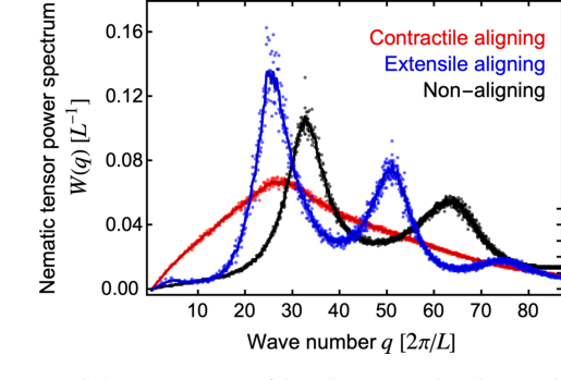 FIG. 9. Power spectrum of the order parameter in active nematic turbulence. Shown is the power spectrum of the nematic tensor, ˆqαβ = nαnβ −1/2 δαβ, in the contractile flow-aligning (Sν = +1.1, red), extensile flow-aligning (Sν = −1.1, blue), and nonaligning (ν = 0, black) cases. For the definition of W (q), see Eq. (B11). Lines represent a smoothed (Gaussian) interpolation of the com- puted data points. Parameter values are as in Fig. 1 and Fig. S1 of the Supplemental Material [35]. For arrested turbulence (blue), this spectrum features a narrow peak with its associated harmonics. For strong large-scale turbulence (red), such peaks are washed out. In all regimes, low-q correlations are essentially absent
Mathematical & Logical Mechanism
The Master Equation
The fundamental behavior of active nematic turbulence, particularly in the defect-free regime studied in this paper, is governed by the interplay between fluid flow and the orientation of the nematic liquid crystal. This interaction is captured by two coupled partial differential equations: one describing the momentum balance of the fluid, which, after non-dimensionalization and taking its curl, becomes a Poisson equation for the stream function, and another describing the dynamics of the nematic director field.
The non-dimensionalized momentum balance equation (derived from the curl of the Navier-Stokes-like equation at vanishing Reynolds number) is:
$$
\nabla^4\psi = -S\partial_\alpha\partial_\beta\tilde{g}_{\alpha\beta} + R\nu\partial_\alpha\partial_\beta(\tilde{g}_{\alpha\beta}h_\parallel - \tilde{g}_{\alpha\beta}h_\perp) \quad \text{(6)}
$$
The non-dimensionalized director dynamics equation (describing how the nematic orientation changes over time) is:
$$
\partial_t\theta - \epsilon_{\alpha\beta}\partial_\alpha\psi \partial_\beta\theta + \frac{1}{A}\nabla^2\theta = h_\parallel + \nu\tilde{g}_{\alpha\beta}\partial_\alpha\partial_\beta\psi \quad \text{(8)}
$$
These two equations, (6) and (8), form the mathematical engine of the defect-free active nematic model. They are coupled because the fluid flow (represented by $\psi$) influences the nematic director ($\theta$), and the nematic director's configuration influences the fluid flow.
Term-by-Term Autopsy
Let's dissect each component of these master equations to understand their mathematical meaning and physical role.
Equation (6): Momentum Balance
$$ \nabla^4\psi = -S\partial_\alpha\partial_\beta\tilde{g}_{\alpha\beta} + R\nu\partial_\alpha\partial_\beta(\tilde{g}_{\alpha\beta}h_\parallel - \tilde{g}_{\alpha\beta}h_\perp) $$
-
$\nabla^4\psi$:
- Mathematical Definition: This is the biharmonic operator acting on the stream function $\psi$. It's equivalent to $\nabla^2(\nabla^2\psi)$. Since $\omega = -\nabla^2\psi$ (vorticity), this term is effectively $-\nabla^2\omega$.
- Physical/Logical Role: In fluid dynamics, this term represents the viscous dissipation of vorticity. It acts as a damping mechanism, resisting changes in the fluid flow and tending to smooth out velocity gradients. The use of $\nabla^4$ (instead of just $\nabla^2$) arises from taking the curl of the momentum balance equation twice to eliminate pressure and express everything in terms of the stream function.
- Why $\nabla^4$: This operator naturally emerges from taking the curl of the Stokes equation (momentum balance at low Reynolds number) when expressed in terms of the stream function. It ensures that the fluid flow remains incompressible and accounts for viscous forces.
-
$S$:
- Mathematical Definition: A dimensionless parameter, $S = \text{sign}(\zeta)$, where $\zeta$ is the active stress parameter.
- Physical/Logical Role: This parameter dictates the nature of the active stress. $S = +1$ for extensile stresses (e.g., rod-like components pushing outwards) and $S = -1$ for contractile stresses (e.g., motor proteins pulling inwards). It's a key control parameter for the system's behavior, influencing whether the system exhibits strong turbulence or dynamical arrest.
- Why a sign: The sign captures the fundamental difference in how active components generate stress, which has profound implications for the resulting flow patterns.
-
$\partial_\alpha\partial_\beta\tilde{g}_{\alpha\beta}$:
- Mathematical Definition: This is the divergence of the nematic orientation tensor $\tilde{g}_{\alpha\beta}$. The tensor $\tilde{g}_{\alpha\beta}$ is defined as $\tilde{g}_{\alpha\beta} = n_\alpha n_\beta - \frac{1}{2}\delta_{\alpha\beta}$, where $n_\alpha$ is a component of the nematic director $\mathbf{n} = (\cos\theta, \sin\theta)$, and $\delta_{\alpha\beta}$ is the Kronecker delta.
- Physical/Logical Role: This term represents the active stress generated by the nematic components. Active nematics internally convert chemical energy into mechanical work, generating stresses that drive fluid flow. The divergence of $\tilde{g}_{\alpha\beta}$ captures how these stresses are distributed and how they drive fluid motion.
- Why divergence: The divergence of a stress tensor (like $\sigma^A$) represents the force density exerted by that stress on the fluid. This is a standard way to couple stress to fluid momentum.
-
$R$:
- Mathematical Definition: The dimensionless viscosity ratio, $R = \gamma/\eta$.
- Physical/Logical Role: This parameter compares the rotational viscosity ($\gamma$) of the nematic director to the shear viscosity ($\eta$) of the fluid. It influences how easily the nematic director reorients in response to flow and elastic torques.
- Why a ratio: It's a ratio because it compares two different types of viscous resistance within the system, crucial for understanding the balance between director rotation and fluid flow.
-
$\nu$:
- Mathematical Definition: The dimensionless flow-alignment parameter.
- Physical/Logical Role: This parameter characterizes the tendency of the liquid crystal director to reorient under shear flow. If $\nu < 0$, the nematic tends to align with the flow (flow-aligning regime). If $\nu > 0$, it tends to tumble (tumbling regime). This parameter is central to the paper's findings on dynamical arrest.
- Why a coefficient: It's a coefficient that scales the strength of the flow-alignment effect, which is a key material property of liquid crystals.
-
$\partial_\alpha\partial_\beta(\tilde{g}_{\alpha\beta}h_\parallel - \tilde{g}_{\alpha\beta}h_\perp)$:
- Mathematical Definition: This term represents the divergence of stresses arising from flow alignment and Ericksen stresses. $h_\parallel$ and $h_\perp$ are components of the orientational field $h_\alpha$, defined in Eq. (7) as $h_\parallel = \frac{1}{A}\nabla^2\theta$ and $h_\perp = \nu(\sin 2\theta d_1\psi + \cos 2\theta d_2\psi)$, where $d_1 = \frac{1}{2}(\partial_x^2 - \partial_y^2)$ and $d_2 = \partial_x\partial_y$. The full $h_\alpha$ is the elastic torque on the director.
- Physical/Logical Role: This term captures the elastic stresses (Ericksen stress) and stresses due to flow alignment. The elastic stresses arise from distortions in the nematic director field, while flow alignment describes how the nematic director reorients in response to the fluid's extensional flow. These stresses feed back into the fluid momentum balance, influencing the flow field.
- Why a difference: The specific combination $\tilde{g}_{\alpha\beta}h_\parallel - \tilde{g}_{\alpha\beta}h_\perp$ arises from the symmetric part of the deviatoric stress tensor (Eq. 4), which includes contributions from elastic torques and flow alignment. The divergence of this tensor represents the force density on the fluid.
Equation (8): Director Dynamics
$$ \partial_t\theta - \epsilon_{\alpha\beta}\partial_\alpha\psi \partial_\beta\theta + \frac{1}{A}\nabla^2\theta = h_\parallel + \nu\tilde{g}_{\alpha\beta}\partial_\alpha\partial_\beta\psi $$
-
$\partial_t\theta$:
- Mathematical Definition: The partial derivative of the nematic angle $\theta$ with respect to time $t$.
- Physical/Logical Role: This is the time evolution term, representing how quickly the nematic director's orientation changes at a fixed point in space. It's the core of the dynamics.
- Why a derivative: It's a fundamental component of any dynamical equation, describing the rate of change of a state variable.
-
$\epsilon_{\alpha\beta}\partial_\alpha\psi \partial_\beta\theta$:
- Mathematical Definition: This is the convective term, representing the advection of the nematic angle $\theta$ by the fluid flow. $\epsilon_{\alpha\beta}$ is the Levi-Civita (totally antisymmetric) tensor, and $\partial_\alpha\psi$ represents components of the fluid velocity $\mathbf{v}$.
- Physical/Logical Role: This term describes how the nematic director is carried along by the fluid flow. If a fluid element moves, it takes its nematic orientation with it. This is a crucial non-linear term that couples the director dynamics to the fluid velocity.
- Why $\epsilon_{\alpha\beta}$ and multiplication: The Levi-Civita tensor is used to form the curl of the stream function, which gives the velocity components. The term $\mathbf{v} \cdot \nabla\theta$ represents the material derivative, capturing changes due to both local time evolution and transport by flow.
-
$\frac{1}{A}\nabla^2\theta$:
- Mathematical Definition: The Laplacian of the nematic angle $\theta$, scaled by the inverse of the activity number $A$.
- Physical/Logical Role: This term represents the elastic torque that resists spatial variations (distortions) in the nematic director field. It tends to smooth out sharp changes in orientation, acting like a restoring force. The activity number $A = L^2/l_a^2$ compares the system size $L$ to the active length $l_a = \sqrt{K/(|\zeta|R)}$, which is the balance between active and elastic nematic stresses. A larger $A$ means elastic forces are relatively weaker compared to active forces.
- Why $\nabla^2$: The Laplacian is the standard mathematical operator for diffusion or elastic forces that tend to minimize spatial gradients.
-
$h_\parallel$:
- Mathematical Definition: The parallel component of the orientational field $h_\alpha$, which is related to the Frank free energy. Specifically, $h_\parallel = \frac{1}{A}\nabla^2\theta$ (from Eq. (7) and context of Eq. (8)).
- Physical/Logical Role: This term represents the elastic torque acting on the director, driving it towards a state of minimal elastic distortion. It's the same elastic restoring force as the $\frac{1}{A}\nabla^2\theta$ term on the LHS, but here it's explicitly shown as a source term. The paper's formulation in (8) effectively combines the elastic torque terms.
- Why addition: The terms on the RHS are sources or sinks of director rotation, contributing to the overall change in $\theta$.
-
$\nu\tilde{g}_{\alpha\beta}\partial_\alpha\partial_\beta\psi$:
- Mathematical Definition: The flow-alignment term, scaled by the flow-alignment parameter $\nu$ and involving the nematic orientation tensor $\tilde{g}_{\alpha\beta}$ and second derivatives of the stream function $\psi$.
- Physical/Logical Role: This term describes the reorientation of the nematic director due to extensional flow (shear). It captures how the fluid's deformation field (related to $\partial_\alpha\partial_\beta\psi$) causes the nematic rods to align or tumble, depending on the sign of $\nu$. This is a crucial coupling term.
- Why multiplication: It's a product of the flow-alignment parameter, the nematic orientation, and the strain-rate tensor (derived from $\partial_\alpha\partial_\beta\psi$), reflecting how these factors combine to produce a reorienting torque.
Key Dimensionless Parameters:
- $L$: System size (length scale).
- $\tau_a = \eta/|\zeta|$: Active time scale.
- $K$: Frank elastic constant.
- $\eta$: Shear viscosity.
- $\gamma$: Rotational viscosity.
- $\zeta$: Active stress parameter.
- $A = L^2/l_a^2 = RL^2|\zeta|/K$: Activity number. Compares system size to active length $l_a$. A large $A$ indicates strong active forcing relative to elastic resistance.
- $R = \gamma/\eta$: Viscosity ratio.
- $\nu$: Flow-alignment parameter.
Step-by-Step Flow
Imagine a single, abstract data point representing the state of the active nematic system at a particular location and time. This state is primarily defined by the local nematic director angle $\theta$ and the fluid stream function $\psi$. The system evolves iteratively through a numerical simulation, like a mechanical assembly line processing these data points.
-
Initial State Input: At a given time step $n$, we have the current nematic angle field $\theta^n$ and stream function field $\psi^n$ across the entire spatial grid.
-
Momentum Balance Calculation (Equation 6 / A1):
- The system first focuses on updating the fluid flow. It takes the current nematic angle $\theta^n$ and uses it to calculate the active stresses (the $S(d_1 \sin 2\theta^n + d_2 \cos 2\theta^n)$ term) and the flow-alignment/Ericksen stresses (the $-\frac{R\nu}{A}(d_1 \cos 2\theta^n \nabla^2\theta^n - d_2 \sin 2\theta^n \nabla^2\theta^n)$ term, which is part of the RHS of (A1)). These terms act as "forcing functions" that drive the fluid.
- These forcing functions are then fed into the momentum balance equation, which is a biharmonic equation for $\psi$. This equation is solved using a pseudospectral method. This means the spatial derivatives are computed very efficiently in Fourier space.
- Crucially, the $G(\theta^n, \psi^n)$ term on the LHS of (A1) (which is part of the flow-alignment stress) depends on $\psi$ itself. To handle this, a fixed-point iteration is used: an initial guess for $\psi$ (often from the previous time step) is used to calculate $G$, then the equation is solved for a new $\psi$. This process repeats until the calculated $\psi$ converges to a stable value for the current time step, ensuring self-consistency between the flow and the stresses it generates.
- Once $\psi^n$ is determined, auxiliary flow fields like velocity components ($v_x, v_y$), vorticity ($\omega$), and flow-alignment rotations ($C^n$) are computed from $\psi^n$.
-
Director Dynamics Calculation (Equation 8 / A4):
- Next, the system turns its attention to updating the nematic director. It takes the newly computed flow fields ($v_x, v_y$) and the current nematic angle $\theta^n$.
- The director dynamics equation (8) describes how $\theta$ changes. The convective term ($\epsilon_{\alpha\beta}\partial_\alpha\psi \partial_\beta\theta$) dictates how the director is advected by the fluid flow. The elastic term ($\frac{1}{A}\nabla^2\theta$) acts to smooth out director distortions. The RHS terms ($h_\parallel + \nu\tilde{g}_{\alpha\beta}\partial_\alpha\partial_\beta\psi$) represent elastic torques and reorientation due to extensional flow.
- This equation is solved using a finite-element method. The convective term is handled separately using a characteristics-Galerkin method for stability, effectively tracing the path of fluid elements. The elastic (Laplacian) term is treated implicitly, meaning it's solved for simultaneously with the new $\theta^{n+1}$ to ensure numerical stability, especially for stiff problems.
- The result is the updated nematic angle field $\theta^{n+1}$.
-
Advance Time Step: The system then increments the time from $n$ to $n+1$, and the entire process repeats, using $\theta^{n+1}$ and $\psi^{n+1}$ as the new inputs.
This iterative, coupled process allows the system to evolve, with fluid flow and nematic orientation continuously influencing each other, leading to the complex patterns and dynamical states observed, such as active turbulence or the arrested patterns.
Optimization Dynamics
The "optimization dynamics" in this context refers less to a traditional machine learning optimization (like gradient descent minimizing a loss function) and more to the iterative numerical solution and the long-term physical evolution of the system towards a stable or quasi-stable state.
-
Numerical Convergence at Each Time Step:
- Fixed-Point Iteration for Stream Function: Within each time step, the momentum balance equation (A1) for the stream function $\psi$ is solved iteratively using a fixed-point method. This means that an initial guess for $\psi$ is used to calculate the non-linear terms, then a new $\psi$ is computed. This new $\psi$ then becomes the input for the next iteration, and the process repeats until the difference between successive $\psi$ solutions falls below a small computational tolerance (e.g., $10^{-8}$). This ensures that the fluid flow field is self-consistent with the stresses generated by the nematic director at that instant. The "loss landscape" here is the residual error of the equation, and the iterations aim to find its "minimum" (zero residual).
- Implicit Treatment for Director Dynamics: For the director dynamics equation (A4), the Laplacian (elastic) term is treated implicitly. This means that the value of $\theta$ at the next time step, $\theta^{n+1}$, is solved for directly, rather than being explicitly calculated from $\theta^n$. This approach enhances numerical stability, especially when dealing with stiff terms (like elastic forces that can cause rapid changes if not handled carefully). It effectively "converges" to a stable $\theta^{n+1}$ that satisfies the equation given the current flow.
-
Physical System Evolution and "Learning":
- Iterative State Update: The entire simulation progresses by iteratively updating the fields $\theta$ and $\psi$ from one time step to the next. This continuous feedback loop between flow and director dynamics drives the system's evolution.
- Loss Landscape (Implicit): While not explicitly defined as a loss function, the system's dynamics can be thought of as navigating a complex "energy landscape" (e.g., Frank free energy, bulk free energy). The system naturally evolves towards states that minimize these energies or, in active systems, reaches dynamically sustained non-equilibrium states.
- Gradients and Driving Forces: The various terms in the equations act as "gradients" or driving forces. For example, the active stress term ($S\partial_\alpha\partial_\beta\tilde{g}_{\alpha\beta}$) drives fluid motion, while the elastic terms ($\nabla^2\psi$ and $\nabla^2\theta$) act as restoring forces, trying to smooth out distortions. The flow-alignment term ($\nu\tilde{g}_{\alpha\beta}\partial_\alpha\partial_\beta\psi$) dictates how the director reorients in response to flow, shaping the system's response.
- Convergence to Dynamical Arrest: The paper's central finding is that, for specific parameter regimes (e.g., extensile aligning nematics with $S\nu < -1$), the system "converges" to a dynamically arrested state. This isn't an optimization in the sense of finding a global minimum, but rather the system settling into a stable, non-equilibrium pattern (treelike domain wall networks) where the chaotic flows are suppressed, and the dynamics become very slow, resembling ageing phenomena in glassy systems. The system "learns" to form these stable patterns through the continuous interplay of active forcing, viscous dissipation, elastic torques, and flow alignment. The "gradients" effectively guide the system into these arrested configurations.
- Role of Noise: Small-amplitude Gaussian white noise is added to the director dynamics (Appendix A.4) to speed up the evolution towards fully developed active turbulence. This noise acts as a perturbation, helping the system explore the "landscape" and escape potential local minima or metastable states, ensuring it reaches the characteristic turbulent or arrested regimes.
In essence, the "optimization" is the physical system's natural tendency to evolve under these governing equations, driven by active forces and constrained by material properties, until it reaches a characteristic dynamic or arrested state. The numerical methods ensure that this evolution is accurately and stably simulated.
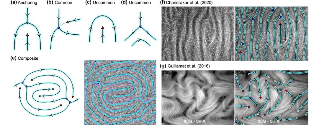 FIG. 4. Motifs of arrested wall networks and experimental snapshots of microtubule-kinesin active nematics. In all diagrams, lines, nodes, and colors are as defined in Fig. 3. (a)–(d) Basic network motifs. The anchoring motif [panel (a)] is made of an endpoint and branchpoint that meet head-on, with the endpoint trapped between the two outgoing walls of the branchpoint. In the motif depicted in panel (b), the endpoint meets the branchpoint from one of its sides, i.e., between the incoming wall and an outgoing wall. The dashed line traces a weak distortion, indicating that the wall associated with the endpoint tends to align its direction with the outgoing wall on the opposite side of the branchpoint. The motifs shown in panels (c) and (d) involve a single pseudodefect interacting with a bare wall. These, along with panel (b), do not follow the tendency to have strictly antiparallel walls. (e) Composite motif schematic (left) and one formed spontaneously in a simulation (right). The stream plot on the right represents the flow, with black indicating maximal |v| and full transparency indicating |v| = 0. The gray background is the line-integral-convolution representation of the nematic director n. Parameter values and color legend for splay and bend distortions are as in Fig. 1(f). (f), (g) Raw fluorescence images from experiments (left panels) and overlaid schematic drawings (right panels) depicting domain walls, pseudodefects, and actual ±1/2 defects in white. (f) Taken from a movie in Ref. [50] (courtesy of Guillaume Duclos), which shows the evolution of the microtubule-based nematic following the bending instability of the aligned state. (g) Taken from a movie in Ref. [51] (courtesy of Pau Guillamat), which shows a turbulent transient with all types of pseudodefects and actual nematic defects. Note how walls may also originate from true +1/2 defects and be absorbed by true −1/2 defects
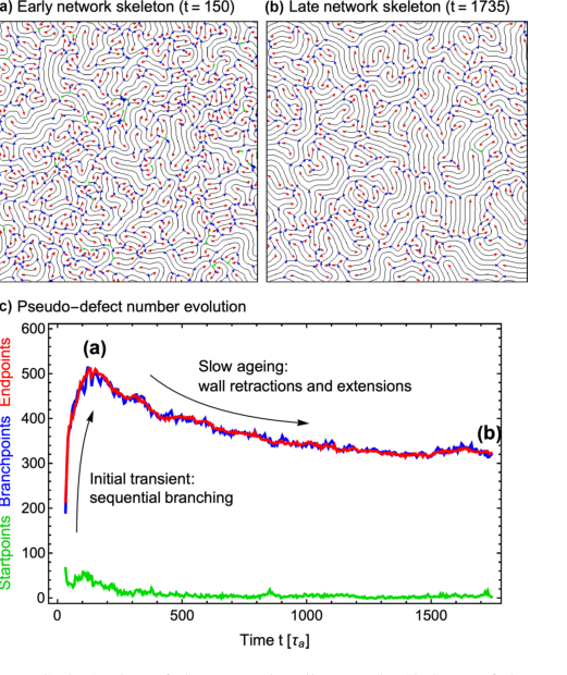 FIG. 5. Ageing of the arrested wall network. Skeleton of the domain walls (black) with startpoints, branchpoints, and endpoints (green, blue, and red triangular nodes) at an early time [panel (a)] and a late time [panel (b)]. The detection of the network skeleton and its nodes is described in Appendix E (Fig. 13). (c) Evolution of the number of startpoints (green), branchpoints (blue), and endpoints (red). In the initial transient, sequential “zigzag” instabilities result in the proliferation of both branchpoints and endpoints. Once the wall pattern establishes a wavelength, the system ages slowly as some endpoints retract and annihilate with their connected branchpoint, while others extend (Movie S5 of the Supplemental Material [35]). Throughout the simulation, there are frequent transitions between branchpoints and startpoints, though the number of startpoints re- mains low. Additionally, the detection algorithm is not perfect, occasionally misidentifying endpoints or branchpoints as startpoints and vice versa. Parameter values were set to R = 1, S = 1, ν = −0.9, and A = 3.2 × 10⁵
Results, Limitations & Conclusion
Experimental Design & Baselines
The authors meticulously designed their numerical experiments to rigorously investigate the dynamics of active nematic turbulence, particularly focusing on the role of topological defects and flow alignment. Their primary tool was large-scale numerical simulations, employing two main models:
First, a director-based defect-free model was utilized, which generalized previous work by incorporating flow alignment and Ericksen stress. This model, governed by equations (6)–(8), inherently precludes the formation of topological defects by enforcing a continuous director field with a fixed modulus. This architectural choice was crucial for isolating the dynamics of domain walls without the confounding influence of defects. Key dimensionless parameters in this model included the activity number $A = L^2/l_a^2$, the viscosity ratio $R = \gamma/\eta$, and the flow-alignment parameter $\nu$. For most simulations, $R=1$ and $A=3.2 \times 10^5$ were set, a regime known to exhibit large-scale active turbulence when $\nu=0$. The experiments were specifically architected to compare two distinct regimes:
1. Contractile flow-aligning (Sv > 1), exemplified by $S=-1$ (contractile stress) and $\nu=-1.1$ (flow-aligning rods). This served as a baseline for "strong large-scale turbulence."
2. Extensile flow-aligning (Sv < -1), with $S=+1$ (extensile stress) and $\nu=-1.1$. This regime was hypothesized to exhibit "arrested turbulence."
A reference case with $\nu=0$ (non-aligning) was also included, where contractile and extensile stresses are equivalent up to a rotation, providing a neutral baseline for comparison.
Second, an unconstrained Q-tensor model was employed to broaden the context of their findings and explore the transition to defect-laden dynamics. This model, based on the Landau-de Gennes framework (Beris-Edwards model) detailed in Appendix D, explicitly allowed for the nucleation of true $\pm 1/2$ topological defects. A crucial control parameter here was the ratio of the defect core size $\epsilon$ to the active length $l_a$. Simulations with this model used parameters $R=1$, $S=1$, $A=10000$, and $\nu=-1$, starting from a quiescent nematic state with a small angular perturbation.
The numerical integration relied on a hybrid scheme, combining a pseudospectral method for momentum balance (Eq. (6)) with a finite-element method (FEM) for the angle field evolution (Eq. (8)), as described in Appendix A. Small-amplitude Gaussian white noise was introduced to accelerate the evolution towards fully developed active turbulence. The "victims" (baseline models) that the authors sought to differentiate from or defeat were primarily the $\nu=0$ non-aligning case and the strong large-scale turbulence observed in the contractile flow-aligning regime. The Q-tensor model also served as a rigorous test for the robustness of the defect-free model's predictions.
What the Evidence Proves
The evidence presented in this paper definitively proves that defect-free active nematic turbulence can undergo a striking dynamical arrest, characterized by the emergence of a stable, treelike network of nematic domain walls that channels coherent flows and suppresses chaotic motion.
The core mechanism of dynamical arrest was ruthlessly proven by comparing the extensile flow-aligning regime (Sv < -1) against the contractile flow-aligning regime (Sv > 1) and the $\nu=0$ reference case. In the contractile aligning regime, simulations (Fig. 1a-1c, Movie S1) showed highly chaotic flows with strong, transient large-scale jets and fragmented, dynamically reorganizing nematic domain walls. This represented the baseline of "strong large-scale turbulence." In stark contrast, the extensile aligning regime (Fig. 1d-1f, Movie S2) exhibited significantly weaker large-scale flows, with dominant flows localized along bending domain walls. Crucially, these domain walls were strongly stabilized, growing and branching into a persistent, space-filling treelike pattern that became "gridlocked" – a state termed dynamical arrest.
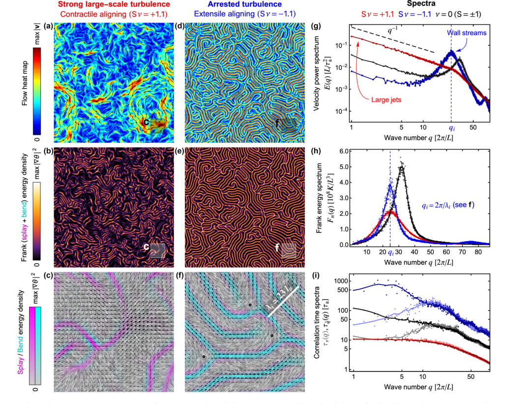 FIG. 1. Strong and arrested regimes of active nematic turbulence. Snapshots from simulations of defect-free active nematic turbulence in contractile [panels (a)–(c)] and extensile [panels (d)–(f)] flow-aligning systems. Parameter values were set to R = 1, ν = −1.1, and A = 3.2 × 10⁵. Top panels (a) and (d) show the flow field; black curves are streamlines, and the color indicates the speed (see Movies S1 and S2 of the Supplemental Material [35]). Middle panels (b) and (e) show the Frank free energy density ∼|∇θ|2, with high-intensity lines corresponding to nematic domain walls (see Movies S1 and S2 of the Supplemental Material [35]). Bottom panels (c) and (f) are zooms highlighting the type of nematic distortion as well as the interplay between nematic walls and flows. The gray-scale background is the line integral convolution representation of the director field n. Magenta and cyan intensities, respectively, represent splay (∇· n)2 and bend |∇× n|2 contributions to the Frank energy density. The black arrows represent the flow field v, which localizes along the nematic walls in the arrested regime. Black circles indicate stagnation points of the flow. White scale bar represents the selected wavelength λi. (g)–(i) Spectra characterizing fully developed active nematic turbulence (see details in Appendix B). The lines in panels (h) and (i) represent a smoothed (Gaussian) interpolation of the computed data points. We compare the flow-aligning contractile [red, as in panels (a)–(c) and Movie S1 of the Supplemental Material [35]] and extensile [blue, as in panels (d)–(f) and Movie S2 of the Supplemental Material [35]] cases with the ν = 0 case (black, as in Fig. S1 and Movie S3 of the Supplemental Material [35]), for which contractile and extensile stresses are equivalent up to a rotation [38,42,43]. (g) Velocity power spectrum on a log-log scale, showing (1) the universal low-q scaling law and (2) the distinct organization of flows across scales in the different cases. The wider scaling regime in the contractile case captures the strong large-scale jets [see panel (a)]. The peak in the extensile case is representative of wall streams [see panel (d)]. (h) Frank energy spectrum, showing that (1) the selected wavelength (peak position) depends on ν but not on the sign of active stress and (2) the peak width depends on the sign of active stress when ν ̸= 0. (i) Spectrum of correlation times associated with the flow v (light colored points and lines) and the nematic tensor ˆqαβ (darker points and lines). This log-log plot reveals strong differences in decay times between the regimes, as well as the differences between the flow and nematic tensor within a regime. Correlation times are extracted from exponential fits to the corresponding space-time autocorrelation functions in Fourier space (see Appendix B)
The definitive, undeniable evidence for this arrest came from the spectral analysis (Fig. 1g-1i):
* Velocity Power Spectrum (Fig. 1g): While both regimes displayed the universal $q^{-1}$ scaling at low wave numbers, the contractile case showed a broad range of scales associated with large-scale jets. The arrested extensile case, however, had a narrower $q^{-1}$ range and a distinct peak at shorter length scales, confirming the dominance of localized wall streams over large-scale chaotic flows.
* Frank Energy Spectrum (Fig. 1h): The extensile (arrested) case showed a much narrower and sharper peak, indicating a highly organized and stable wall pattern, unlike the broader peak in the chaotic contractile regime.
* Correlation Time Spectra (Fig. 1i): This was perhaps the most compelling evidence. The arrested regime exhibited significantly longer correlation times for both the flow and nematic tensor fields, especially at large scales. This directly quantified the reduced dynamics and the "locking" of the pattern, proving that the system had indeed undergone dynamical arrest.
Further evidence highlighted the emergent topology of these arrested states. The domain walls formed "pseudodefects" (startpoints, branchpoints, endpoints) that, while not true topological defects, carried a conserved pseudocharge (Fig. 3). The simulations illustrated the dynamic evolution from initial striped patterns, through zigzag instabilities and wall branching, to the final gridlocked treelike pattern (Fig. 2).
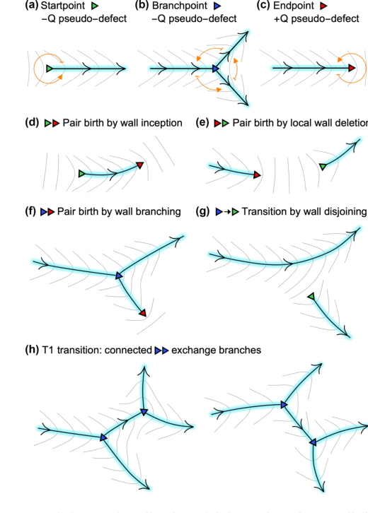 FIG. 3. Domain wall nodes and their pseudotopology. In all di- agrams, black directed lines represent nematic bending walls, with gray lines tracing the director and cyan indicating the bending energy. (a)–(c) Nodes are either startpoints (green, negative pseudodefects), branchpoints (blue, negative pseudodefects), or endpoints (red, posi- tive pseudodefects). The orange curves illustrate the paths excluding walls used to define the pseudocharge (Appendix C). (d)–(e) Two ways in which a startpoint-endpoint pair of opposite charge can be born. The inverse processes of (d) [complete wall dissolution] and (e) [local wall completion] result in the annihilation of such pairs. (f) Wall branching gives birth to a branchpoint-endpoint pair, also of opposite charge. A connected pair may annihilate via branch retraction. (g) A branchpoint [panel (b)] transitions into a startpoint when one outgoing wall disjoins. The inverse process corresponds to a startpoint [panel (a)] joining with a bare wall. (h) Connected branchpoints can shrink their connecting branch, transiently creat- ing a −2Q pseudocharged structure, exchange outgoing walls, and extend again in the perpendicular direction. The processes depicted in panels (d)–(h) are further illustrated in Animations S1–S5 of the Supplemental Material [35]
The "anchoring motif" (Fig. 4a), a specific arrangement of pseudodefects, was identified as a particularly stable structure, acting as a "trap" for flow. The slow relaxation of the pseudodefect number over long timescales (Fig. 5c), reminiscent of aging in glassy systems, further underscored the arrested nature of the state. Moreover, the arrested patterns were shown to enclose "unicursal labyrinths" (Fig. 6b), a rare pattern in other systems, demonstrating a unique pattern-formation phenomena.
The robustness of dynamical arrest was then validated using the Q-tensor model. This model confirmed that arrest is not an artifact of the defect-free constraint but a generic feature when defect nucleation is energetically suppressed (i.e., small $\epsilon/l_a$). As the defect core size $\epsilon$ was increased beyond a critcal threshold ($\approx 0.25 l_a$), true $\pm 1/2$ defects began to nucleate (Fig. 7b, 7e, 7f), disrupting the arrested wall patterns and transitioning the system into a disordered, vortex-dominated turbulent state.
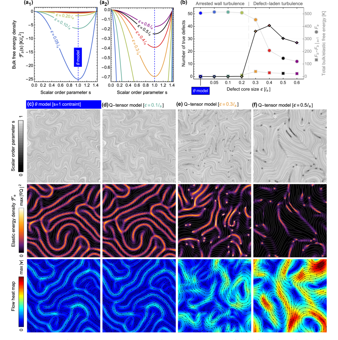 FIG. 7. Persistence of dynamical arrest and the transition to defect-laden turbulence. (a) Plots of the bulk free energy as a function of the scalar order parameter s for the values of ϵ explored in our simulations. Dashed blue line represents the θ model, for which s = 1 is enforced. The energy is shown in units of K/ℓ2 a, characterizing elastic distortions. Note the difference in magnitude between panel (a1), highlighting cases for which defects do not form, and panel (a2), for which they do. (b) Statistical means of the total defect number (diamond markers, black line), the total bulk free energy (square markers, gray line), and total elastic free energy (circle markers, gray line), as a function of ϵ. These temporal averages characterize the fully developed turbulent state in our simulations (discarding initial transients). For timeseries and more detailed statistical breakdown, see Fig. 12. Typical snapshots from simulations of the θ model [panel (c)] and the full Q-tensor model, at increasing values of ϵ [panels (d)–(f)]. Top panels show the line integral convolution (LIC) representation of the director field n, overlaid with a density plot of the scalar order parameter s, such that s = 0 is black and s = 1 is transparent (revealing the gray-scale LIC texture). True topological defects are seen as black spots and s/2, n are computed as the principal eigenpair of Q. Panels of the center row show the elastic energy density along with white traces of n. Bottom panels show the flow heatmap with black streamlines. In all simulations depicted here, we fixed R = 1, S = 1, A = 10 000, ν = −1 (the extensile rod-aligning regime), and set the same initial condition: a quiescent nematic state (s = 1) with a small angular perturbation. See also Movies S6 and S7 of the Supplemental Material [35]
This transition was accompanied by a dramatic reduction in the total elastic free energy (Fig. 7b, 12c), as defects efficiently dissolved the high-energy domain walls. The simulations also revealed that branchpoint pseudodefects acted as "hot spots" for defect nucleation (Movie S8), establishing a clear link between the defect-free and defect-laden regimes. The quantitative agreement between the Q-tensor model and the constrained $\theta$ model at small $\epsilon/l_a$ (Fig. 11, Movie S6) further solidified the validity of the defect-free approach in that limit.
Limitations & Future Directions
While this work provides profound insights into active nematic turbulence, it also highlights several limitations and opens numerous avenues for future research.
One significant limitation is the experimetal realization of dynamical arrest. The paper explicitly states that this primary prediction has not yet been observed in experiments. Achieving this would require active materials where the energetic cost of nucleating defect pairs is substantially higher than in current experimental setups. This points to a need for materials science innovation, perhaps involving new molecular designs or environmental controls that suppress defect formation.
Another area for further exploration concerns system size effects. While large-scale simulations were performed, the authors note that in even larger systems, frequent fracturing events prevented the persistent, system-spanning connectivity of the arrested wall network (Movie S9). This suggests that there might be a critical system size beyond which the arrested state becomes unstable, potentially due to the increasing strength of chaotic large-scale flows that could disrupt the wall network. Future work should aim to map out this stability boundary and understand the mechanisms of fracture at very large scales.
The nonlinear wavelength selection mechanism remains an open question. The paper acknowledges that this mechanism, balancing coarsening and bending/folding of walls, is inherently nonlinear and two-dimensional, and its precise dependence on various parameters is not yet fully understood. Deeper theoretical and computational studies are needed to unravel this complex interplay.
Furthermore, the observed non-monotonic dependence of defect density on core size (decreasing with increasing core size in some regimes) is intriguing but not fully explained, being deferred to future work. This suggests a more complex relationship between defect energetics and pattern formation than currently understood. The computational cost of Q-tensor simulations at very small defect core sizes also presents a practical limitation, making the simpler $\theta$ model a necessary alternative in that regime.
Looking ahead, several discussion topics emerge:
- Designing Defect-Free Active Nematic Systems: How can we leverage the understanding of flow alignment and defect core size to engineer active nematic systems that intrinsically suppress defect formation, thereby promoting dynamical arrest? This could involve tuning material properties, activity levels, or confinement geometries.
- Interplay of Pseudodefects and True Defects: The transitional regime where pseudodefects and true topological defects coexist is rich and warrants further investigation. How do true defects, which can act as origin or termination points for walls, interact with the pseudodefect network? Can this interaction be controlled to switch between arrested and turbulent states?
- Nature of Long-Range Topological Order: The unicursal labyrinths observed in the arrested state suggest a form of long-range topological order. What are the mathematical and physical properties of this order? How does it compare to other forms of topological order in condensed matter systems, and what are its implications for material properties?
- Analogies to Glassy Systems and Aging: The slow relaxation dynamics of the arrested wall networks share features with aging phenomena in glassy systems. Can insights from the physics of glasses be applied to better understand the stability, relaxation, and response of arrested active nematics to perturbations?
- Impact of Constituent Depletion: The paper mentions that nematic constituents are observed to be depleted at defects in experiments, which could lower defect energy costs. Incorporating this effect into future models could provide a more accurate picture of defect nucleation and its influence on wall network stability.
- Generalization to Three Dimensions: While this study focused on 2D systems, extending the analysis to three dimensions would be a natural next step. Would similar dynamical arrest phenomena or pseudotopological structures emerge in 3D active nematics, and how would their properties differ?
These future directions underscore the cross-disciplinary nature of this field, requiring collaboration between theoretical physicists, materials scientists, and experimentalists to fully unravel the complexities of active nematic systems.