Amortizing intractable inference in diffusion models for vision, language, and control

Background & Academic Lineage

The Origin & Academic Lineage

This paper's problem precisely originates from the recent success and widespread adoption of diffusion models as powerful generative models across various domains, including computer vision, natural language processing, and reinforcement learning. While these models excel at generating high-quality data by learning to reverse a gradual noising process, their application in downstream tasks often requires a more complex form of inference: sampling from a posterior distribution.

Historically, diffusion models, first introduced in 2015 by Sohl-Dickstein et al. [68], are a class of hierarchical generative models that learn to model complex data distributions. The core idea involves defining a forward diffusion process that gradually adds noise to data, transforming it into a simple, tractable distribution (like Gaussian noise). Then, a neural network is trained to learn the reverse process, effectively denoising the data step by step to generate new samples.

The specific problem emerges when these pretrained diffusion models are used as priors $p(x)$ in scenarios where the desired output must also satisfy an additional, often complex, constraint $r(x)$. This constraint could be a classifier's likelihood (e.g., generating an image of a specific class), a reward function in reinforcement learning (e.g., generating actions that maximize a reward), or a language model's likelihood for infilling missing text. The goal then becomes sampling from the product distribution $p_{\text{post}}(x) \propto p(x)r(x)$, which represents the Bayesian posterior. This problem is particularly challenging because the hierarchical nature of diffusion models makes exact sampling from such posteriors intractable, especially when $r(x)$ is a "black-box" function that doesn't offer easy analytical solutions.

The fundamental limitation or "pain point" of previous approaches is their inability to perform this intractable posterior inference accurately and efficiently. Existing methods typically fall into several categories, each with significant drawbacks:
* Linear approximations or stochastic optimization: These methods often provide only approximate solutions [73, 33, 31, 11, 22, 48], which may not capture the true posterior distribution faithfully.
* Guidance term estimation: Techniques like classifier guidance [12] attempt to estimate a "guidance" term by training a classifier on noised data. However, this approach is limited because it requires specific noised data, and when such data is unavailable, it resorts to approximations or Monte Carlo estimates [70, 14, 10]. These approximations are notoriously difficult to scale to high-dimensional problems, which are common in modern generative tasks.
* Reinforcement learning (RL) methods: Recent RL-based approaches [8, 16] for this problem, while promising, have been shown to be biased and suffer from mode collapse. Mode collapse means the model fails to generate diverse samples, instead getting stuck generating only a few high-reward examples, thus not fully exploring the true posterior distribution. This lack of diversity and accuracy in sampling from the full posterior distribution is a major hurdle for reliable and versatile applications of diffusion models in complex downstream tasks.

Intuitive Domain Terms

Here are a few specialized domain terms from the paper, translated into intuitive analogies:

• Diffusion Models: Imagine you have a very blurry, noisy photograph. A diffusion model is like a skilled digital artist who knows exactly how to gradually remove the blur and noise, step by step, until the original, clear photograph is revealed. It learns this "un-blurring" process by studying how images become noisy in the first place.
• Posterior Inference: Think of it like trying to find a specific type of rare bird. You have a general field guide that tells you about all birds (the "prior" knowledge). But then, you get a tip from a local expert: "This bird only appears near a specific type of tree" (the "constraint"). Posterior inference is the process of combining your general bird knowledge with this new, specific tip to narrow down your search and find the most likely locations for that particular bird.
• Mode Collapse: Picture a chef who is asked to bake a variety of cakes for a party. If the chef only bakes chocolate cakes, even though the party-goers want vanilla, strawberry, and lemon cakes too, that's mode collapse. The chef has "collapsed" onto a single type of cake (chocolate) and isn't exploring the full range of desired options, even if the chocolate cake is very good.
• Relative Trajectory Balance (RTB): Consider a tightrope walker trying to cross a very long, wobbly rope. Instead of just focusing on getting to the other side, which might lead to falling, RTB is like having a sophisticated sensor system that constantly compares the walker's forward movement with a hypothetical backward movement, relative to a stable, known path. This continuous, relative comparison helps the walker maintain perfect balance and reach the destination reliably, without veering off or getting stuck.
• Black-box constraint $r(x)$: Imagine you're playing a video game where you're trying to design a character. You can change various features, but there's a mysterious "judge" who just gives you a score for your character's appeal, without explaining why they gave that score. You can't see inside the judge's mind; you just get a number. This judge is a black-box constraint – you know its output, but not its internal workings.

Notation Table

Notation	Description
$p_{\theta}(x)$	A pretrained diffusion generative model (the prior), parameterized by $\theta$.
$r(x)$	A positive, black-box constraint or likelihood function.
$p_{\text{post}}(x)$	The target posterior distribution, $p_{\text{post}}(x) \propto p_{\theta}(x)r(x)$.
$P_{\Phi}^{\text{post}}(\tau)$	The probability of a trajectory $\tau$ under the posterior diffusion model, parameterized by $\Phi$.
$p_{\theta}(\tau)$	The probability of a trajectory $\tau$ under the prior diffusion model, parameterized by $\theta$.
$\tau = (X_0, X_{\Delta t}, \dots, X_1)$	A diffusion trajectory from initial noise $X_0$ to final data $X_1$.
$X_t$	A data point at an intermediate time step $t$ in the diffusion process.
$u_{\Phi}^{\text{post}}(x_t, t)$	The drift term of the posterior SDE, learned by a neural network with parameters $\Phi$.
$u_{\theta}(x_t, t)$	The drift term of the prior SDE, learned by a neural network with parameters $\theta$.
$\mathcal{L}_{\text{RTB}}(\tau; \Phi)$	The Relative Trajectory Balance (RTB) loss function.
$Z$	A normalization constant for the posterior distribution.
$T$	The total number of discrete time steps in the diffusion process.
$\Delta t$	The duration of a single time step, $\Delta t = 1/T$.
$B$	The accumulation batch size for batched gradient computation.
$E[\log r(x)]$	Expected log reward, a metric for how well samples satisfy the constraint.
FID	Fréchet Inception Distance, a metric for image quality and similarity to a target distribution.
BERTScore	A metric for text generation quality, comparing generated text to reference text.
BLEU-4	A metric for text generation quality, based on n-gram overlap.
GLEU-4	A metric for text generation quality, similar to BLEU but with better correlation to human judgment.

Problem Definition & Constraints

Core Problem Formulation & The Dilemma

The central problem addressed by this paper is the intractable posterior inference in diffusion models when they are used as priors for downstream tasks. Specifically, the authors aim to bridge the gap between having a powerful generative diffusion model as a prior and needing to sample from a constrained version of that prior.

The starting point (Input/Current State) is a pretrained diffusion generative model, denoted as $p_{\theta}(x)$, which effectively models complex data distributions (e.g., images, text, actions). Alongside this prior, there is a black-box constraint or likelihood function, $r(x)$, which represents additional conditions or preferences. The goal is to perform inference on the product of these two distributions.

The desired endpoint (Output/Goal State) is a new, trained diffusion model, $p_{\phi}^{\text{post}}$, that can unbiasedly sample from the true posterior distribution $p_{\text{post}}(x) \propto p_{\theta}(x)r(x)$. This means the trained model should accurately reflect the combined influence of the prior and the constraint, allowing for flexible and accurate conditional generation or policy learning.

The exact missing link or mathematical gap is the inherent intractability of directly sampling from this posterior $p_{\text{post}}(x)$. Diffusion models generate samples through a deep chain of stochastic transformations, making exact sampling from $p_{\theta}(x)r(x)$ under a black-box $r(x)$ intractable. Previous methods either provide only approximate solutions, work in restricted cases, or introduce biases and suffer from issues like mode collapse. The paper attempts to bridge this by proposing a novel training objective, Relative Trajectory Balance (RTB), which, when satisfied, ensures that the trained posterior diffusion model $p_{\phi}^{\text{post}}$ samples from the desired distribution. Mathematically, the paper seeks to train $p_{\phi}^{\text{post}}$ such that it satisfies the relative trajectory balance constraint:
$$Z p_{\phi}^{\text{post}}(X_0, X_{\Delta t}, \dots, X_1) = r(X_1) p_{\theta}(X_0, X_{\Delta t}, \dots, X_1)$$
where $Z$ is a normalization constant, $X_0, \dots, X_1$ represents a denoising trajectory, and $p_{\theta}(X_0, X_{\Delta t}, \dots, X_1)$ is the joint probability of a trajectory under the prior.

The painful trade-off or dilemma that has trapped previous researchers is primarily between accuracy/unbiasedness and tractability/computational efficiency. Existing solutions often fall into one of these traps:
1. Approximation vs. Bias: Methods relying on linear approximations or stochastic optimization are tractable but often yield biased outcomes or are challenging to scale to high-dimensional problems. For example, classifier guidance, while effective in some cases, provides a biased approximation of the true posterior drift.
2. Reward Maximization vs. Mode Coverage: Reinforcement learning (RL)-based methods, which fine-tune diffusion models to maximize a reward function, frequently suffer from mode collapse. They might achieve high rewards by focusing on a few high-reward modes, but at the cost of significantly poorer diversity and an inaccurate representation of the full posterior distribution. This means improving one aspect (reward) often breaks another (diversity).
3. On-policy vs. Off-policy Training: On-policy training, where trajectories are sampled from the current model, can be inefficient and struggle to discover all modes of the posterior. While off-policy exploration can improve mode coverage, it introduces its own set of challenges regarding training stability and sample efficiency.

Constraints & Failure Modes

The problem of amortizing intractable inference in diffusion models is made insanely difficult by several harsh, realistic walls:

• Computational Constraints:

  • Intractability of Exact Posterior Sampling: The fundamental challenge is that exact sampling from the product of a diffusion prior and a black-box constraint $r(x)$ is computationally intractable, especially given the hierarchical nature of diffusion models.
  • High-Dimensionality: Many existing inference techniques, including Monte Carlo estimates and linear approximations, are "challenging to scale to high-dimensional problems" such as those encountered in vision, language, and control tasks.
  • Hardware Memory Limits: For large diffusion models, computing and storing gradients for all steps in a long denoising trajectory is "prohibitive" due to hardware memory limitations. This necessitates memory-efficient techniques like stochastic subsampling or batched gradient computation, which can introduce trade-offs like increased gradient variance.
  • Training Time: The simulation-based training required for learning posterior samplers can be "slow and memory-intensive," as noted in the limitations section. The total estimated compute time for all experiments in the paper is 3000 hours on powerful GPUs, indicating the significant computational cost.

• Data-Driven Constraints:

  • Lack of Unbaised Posterior Samples: Training methods that rely on direct supervision from true posterior samples are often infeasible because such samples are not assumed to be available. For instance, classifier guidance requires a differentiable classifier on noisy data, which is generally not tractable to derive or learn without access to unbiased data.
  • Sparsity of Data for Guidance Term: When data for training a classifier on noised data is unavailable, researchers must resort to approximations, which can introduce bias.
  • Sensitivity to Imperfect Prior Models: The proposed loss function can be sensitive to an "imperfectly fit prior model," which can impact training stability and performance.

• Mathematical & Logical Constraints:

  • Non-differentiable Constraints: The constraint function $r(x)$ is often a "black-box," implying it may not be differentiable, complicating gradient-based optimization. While the paper explores cases where $r(x_1)$ is differentiable, the general problem formulation must account for non-differentiable scenarios.
  • Bias in Approximations: Previous methods, such as classifier guidance or RL with per-step KL regularization, introduce inherent biases that prevent them from asymptotically achieving the true posterior.
  • Mode Collapse: RL-based fine-tuning methods, particularly those without sufficient regularization, are prone to mode collapse, where the model only samples a subset of the true posterior modes, leading to a lack of diversity in generated samples.
  • Intractability of Marginal KL Divergence: In contexts like RL-based fine-tuning for text-to-image generation, the marginal KL divergence between the fine-tuned model and the prior is intractable for diffusion models, forcing reliance on approximations like per-step KL penalties, which can introduce bias.

Why This Approach

The Inevitability of the Choice

The adoption of Relative Trajectory Balance (RTB) was not merely a choice but a necessity driven by the inherent intractability of posterior inference in diffusion models when used as priors for downstream tasks. The paper explicitly states that "Diffusion models have emerged as effective distribution estimators... but their use as priors in downstream tasks poses an intractable posterior inference problem." (Abstract, p.1). The core issue stems from the "hierarchical nature of the generative process in diffusion models," which makes "exact sampling from posteriors $p(x)r(x)$ under a black-box function $r(x)$ intractable" (p.2).

Traditional "SOTA" methods proved insufficient for this specific challenge. Existing approaches either offer only approximate solutions or are limited to restricted cases. For instance, common inference techniques rely on linear approximations [73, 33, 31, 11] or stochastic optimization [22, 48], which inherently introduce approximations. Another popular strategy involves estimating the 'guidance' term by training a classifier on noised data [12]. However, this method falters when such noised data is unavailable, forcing reliance on further approximations or Monte Carlo estimates [70, 14, 10] that are notoriously difficult to scale to high-dimensional problems. Furthermore, recent reinforcement learning (RL) methods [8, 16] proposed for this problem are known to be biased and susceptible to mode collapse, as visually demonstrated in Figure 1 (p.3).

The authors realized that a fundamentally different approach was needed to achieve asymptotically unbiased sampling from these intractable posteriors. This led to the development of RTB, which is derived from the generative flow network perspective on diffusion models. This perspective provides the theoretical underpinning for an objective that can overcome the limitations of prior methods, offering a path to unbiased posterior sampling where other techniques either approximate, fail, or suffer from critical issues like mode collapse.

Comparative Superiority

Relative Trajectory Balance (RTB) demonstrates qualitative superiority over previous gold standards through several structural and operational advantages, extending beyond mere performance metrics.

Firstly, RTB is an "asymptotically unbiased objective that recovers the difference in drifts (and thus the gradient of the log-convolved likelihood) in a data-free manner" (p.5). This is a significant structural advantage over classifier guidance, which, while providing an exact solution for the posterior drift, requires a differentiable classifier on noisy data that is often intractable to derive or learn without unbiased data samples. RTB circumvents this data dependency, offering a more robust and general solution.

Secondly, the method exhibits superior memory efficiency and scalability. A critical insight is that "the gradient of this objective with respect to $\phi$ does not require differentiation (backpropagation) into the sampling process that produced a trajectory x0 → ... → x1" (p.5). This property yields two key benefits:
1. Off-policy optimization: RTB can be optimized as an off-policy objective, meaning trajectories for training can be sampled from a distribution different from the target posterior itself. This flexibility is crucial for "ensuring mode coverage" (p.5) and is a distinct advantage over on-policy RL methods that are prone to mode collapse (Fig. C.2, p.19).
2. Batched gradient accumulation: The gradient computation for RTB does not necessitate storing the entire computation graph for all timesteps. Instead, "only the accumulation batch size B, not the trajectory length T, is constrained by the memory budget" (p.27). This allows for scaling training to a large number of diffusion steps without increasing gradient variance through stochastic subsampling, with training time growing linearly with the number of steps under a fixed memory budget. This dramatically reduces memory complexity, making it overwhelmingly superior for high-dimensional problems where storing full trajectories is prohibitive.

Finally, RTB's versatility is a qualitative strength. The paper showcases its broad applicability across diverse domains, including vision (classifier-guided image generation, text-to-image generation), language (infilling with discrete diffusion LLMs), and continuous control (offline reinforcement learning). This wide range of successful applications underscores its structural advantage in handling various forms of diffusion priors and black-box constraints.

Alignment with Constraints

The chosen RTB method aligns perfectly with the problem's harsh requirements, forming a strong "marriage" between the problem definition and the solution's unique properties.

The primary constraint, as defined in the problem, is the need to sample from "product distributions, where a pretrained diffusion model serves as a prior $p(x)$ that is multiplied by an auxiliary constraint $r(x)$" (p.2). RTB is explicitly designed for "training diffusion models that sample from posterior distributions under a diffusion model prior" (§2.2), directly addressing this core requirement.

Furthermore, the auxiliary constraint $r(x)$ is often a "black-box constraint or likelihood function" (Abstract, p.1), meaning its functional form might be complex or non-differentiable. RTB is formulated to handle "arbitrary positive constraint $r(x_1)$" (p.5) and "arbitrary black-box likelihoods" (p.10), making it highly suitable for scenarios where the constraint function is not easily amenable to traditional gradient-based methods.

The problem also highlights the "intractable posterior inference" (Abstract, p.1) as a major hurdle. RTB provides an "asymptotically unbiased training objective" (p.2), offering a theoretically sound way to tackle this intractability, rather than relying on approximations that can introduce bias.

For conditional problems, where constraints depend on other variables (e.g., $r(x_1; y) = p(y | x_1)$), RTB allows the posterior drift to be conditioned on $y$, enabling "amortized inference" and "generalization to new $y$ not seen in training" (p.5). This property is crucial for practical applications requiring efficient inference across varying conditions.

Lastly, the need to scale to "high-dimensional problems" (p.2) and "large diffusion models" (p.5) imposes significant memory and computational constraints. RTB's memory-efficient training, through batched gradient accumulation and stochastic subsampling, directly addresses these practical limitations. The ability to scale training with a large number of diffusion steps without increasing memory budget, as discussed in §H.1, is a perfect fit for the demanding nature of modern generative models.

Rejection of Alternatives

The paper provides clear reasoning for rejecting several popular approaches for the specific problem of amortizing intractable posterior inference in diffusion models:

• Traditional Inference Techniques (Linear Approximations, Stochastic Optimization): The authors note that "Common solutions to this problem involve inference techniques based on linear approximations [73, 33, 31, 11] or stochastic optimization [22, 48]" (p.2). These methods are deemed insufficient because they "solve only approximately or in restricted cases" (Abstract, p.1), failing to provide the asymptotically unbiased sampling that RTB aims for.

• Classifier Guidance (CG) / Diffusion Posterior Sampling (DPS) / Loss-Guided Diffusion Monte Carlo (LGD-MC): These methods, which attempt to estimate the 'guidance' term, are criticized for several reasons:

  • They "result in biased outcomes" (Fig. 1, p.3).
  • They rely on "training a classifier on noised data [12]," which is problematic "when such data is not available" (p.2).
  • Deriving a differentiable classifier on noisy data is "not, in general, tractable" (p.5), and learning it requires "unbiased data samples," which are precisely what the problem aims to generate.
  • Experimentally, "Classifier-guidance-based methods, like DP and LGD-MC, exhibit high diversity, but fail to appropriately model the posterior distribution (lowest log r(x))" (p.7). They also achieve "lowers classifier average rewards" and fail to "appropriately model the posterior distribution" (p.21).

• Reinforcement Learning (RL) Methods (e.g., DPOK, DDPO): While RL methods [8, 16] have been proposed for this problem, they suffer from critical flaws:

  • They are "biased and prone to mode collapse (Fig. 1)" (p.2). Figure E.1 (p.20) further illustrates "early mode collapse" and "reward exploitation" in pure RL fine-tuning.
  • "Pure RL fine-tuning (no KL regularization) displays mode collapse characteristics, achieving high rewards in exchange for significantly poorer diversity and FID scores" (p.7).
  • RL methods for fine-tuning diffusion models are typically "on-policy" (p.19), which makes them "prone to mode collapse" (Fig. C.2, p.19).
  • Methods like DPOK and DDPO optimize an upper bound on the marginal KL using a per-step penalty, which introduces bias. RTB, in contrast, "can avoid the bias in such an approximation and directly learn to generate unbiased samples from the posterior $p(x_1 | z)$" (p.7).

The paper does not explicitly discuss the rejection of Generative Adversarial Networks (GANs) for this specific problem. The focus is on improving posterior inference within the diffusion model framework, where diffusion models are already established as the prior. Therefore, a direct comparison or rejection of GANs as an alternative generative model for the prior itself is outside the scope of this particular analysis.

Figure 3. Fine-tuning Stable Diffusion with Im- ageReward. We report mean log 𝑟(x1, z) and diver- sity, measured as the mean cosine distance between CLIP embeddings for a batch of 100 generated im- ages.2

Mathematical & Logical Mechanism

The Master Equation

The absolute core equation that powers this paper is the Relative Trajectory Balance (RTB) loss function. This objective drives the posterior diffusion model to sample from the desired target distribution. The loss is defined as the squared logarithm of a ratio, aiming to bring this ratio to unity.

$$ \mathcal{L}_{\text{RTB}}(\tau; \Phi) := \left( \log \frac{Z P_{\Phi}^{\text{post}}(\tau)}{r(X_1) p_{\theta}(\tau)} \right)^2 $$

Here, $\tau = (X_0, X_{\Delta t}, \dots, X_1)$ represents a full trajectory in the diffusion process. The trajectory probabilities $P(\tau)$ are themselves products of initial distributions and conditional transition probabilities over discrete time steps, as shown in Equation (3) of the paper:

$$ P(\tau) = p(X_0) \prod_{i=1}^T P(X_{i\Delta t} | X_{(i-1)\Delta t}) $$

Term-by-Term Autopsy

Let's dissect the master equation to understand each component's role. For clarity, we'll primarily focus on the term inside the logarithm, as its minimization to zero is the direct goal.

• $\mathcal{L}_{\text{RTB}}$:

  1. Mathematical Definition: The Relative Trajectory Balance (RTB) loss function.
  2. Physical/Logical Role: This is the primary objective function that the model seeks to minimize during training. Driving this loss to zero ensures that the relative trajectory balance constraint (Equation 8 in the paper) is satisfied. This, in turn, guarantees that the posterior diffusion model $P_{\Phi}^{\text{post}}$ learns to sample from the desired target posterior distribution $p_{\text{post}}(x_1) \propto p_{\theta}(X_1)r(X_1)$.
  3. Why squaring? Squaring the log-ratio is a standard technique in loss function design (akin to Mean Squared Error). It ensures the loss is always non-negative and provides a smooth, differentiable objective, which is crucial for gradient-based optimization. It penalizes larger deviations from the target ratio (which is 1) more significantly than smaller ones, encouraging precise convergence.

• $\tau = (X_0, X_{\Delta t}, \dots, X_1)$:

  1. Mathematical Definition: A specific trajectory in the diffusion process, representing a sequence of states from an initial noisy state $X_0$ to the final, denoised data point $X_1$, passing through intermediate states $X_{i\Delta t}$ at discrete time steps.
  2. Physical/Logical Role: This is the fundamental unit of operation for the RTB mechanism. The entire learning process evaluates and adjusts the model based on how well it generates these sequential paths through the data space.

• $\Phi$:

  1. Mathematical Definition: The set of learnable parameters for the posterior diffusion model, $P_{\Phi}^{\text{post}}$. These parameters typically define the drift term $u_{\Phi}^{\text{post}}(x_t, t)$ of the underlying stochastic differential equation (SDE), which is often implemented as a neural network.
  2. Physical/Logical Role: These are the weights and biases of the neural network that govern how the posterior model generates samples. The optimization process adjusts $\Phi$ to align the posterior sampling with the desired target distribution.

• $Z$:

  1. Mathematical Definition: A scalar normalization constant, specifically $Z = \int q(x_1)r(x_1) dx_1$ as derived in Proposition 1. For numerical stability, its logarithm, $\log Z$, is often learned or estimated.
  2. Physical/Logical Role: This term is essential for ensuring that the target posterior distribution $p_{\text{post}}(x_1) \propto p_{\theta}(X_1)r(X_1)$ is correctly normalized. Since the constraint function $r(X_1)$ might be an unnormalized likelihood or reward, $Z$ scales the overall probability to integrate to 1. It's vital for matching the absolute probabilities, not just relative proportions.

• $r(X_1)$:

  1. Mathematical Definition: A positive, black-box constraint function or likelihood function, evaluated at the final data point $X_1$.
  2. Physical/Logical Role: This term represents the "reward" or "guidance" signal that steers the diffusion process towards desired characteristics. For instance, it could be a classifier's likelihood $p(c|X_1)$ for a specific class $c$, or a reward function $\exp(\beta Q(s,a))$ in reinforcement learning. It encodes the specific properties we want the generated data to possess.

• $p_{\theta}(\tau)$:

  1. Mathematical Definition: The probability of a trajectory $\tau$ under the prior diffusion model, parameterized by $\theta$. This is typically a product of the initial distribution $p(X_0)$ and conditional transition probabilities $P_{\theta}(X_{i\Delta t} | X_{(i-1)\Delta t})$ for each step.
  2. Physical/Logical Role: This represents the "baseline" or "unconditional" generative process. It's a pre-trained diffusion model that generates data without any specific constraints. The RTB objective uses this as a reference point to define the relative balance for the posterior model.

• $P_{\Phi}^{\text{post}}(\tau)$:

  1. Mathematical Definition: The probability of a trajectory $\tau$ under the posterior diffusion model, parameterized by $\Phi$. Similar to $p_{\theta}(\tau)$, it's a product of $p(X_0)$ (often shared with the prior) and conditional transition probabilities $P_{\Phi}^{\text{post}}(X_{i\Delta t} | X_{(i-1)\Delta t})$.
  2. Physical/Logical Role: This represents the generative process that we are actively learning to sample from the desired posterior distribution. Its parameters $\Phi$ are updated during training to make its trajectories align with the constraint $r(X_1)$ relative to the prior $p_{\theta}(\tau)$.

• $\log(\cdot)$:

  1. Mathematical Definition: The natural logarithm.
  2. Physical/Logical Role: The logarithm transforms products of probabilities into sums of log-probabilities, which is numerically more stable and often easier to optimize. It also converts ratios of probabilities into differences of log-probabilities, a common technique in information theory (e.g., KL divergence). The objective aims to make the log-ratio zero, meaning the ratio itself is one.

• $\sum_{i=1}^T$:

  1. Mathematical Definition: A summation over discrete time steps $i$ from 1 to $T$.
  2. Physical/Logical Role: This operator aggregates the log-ratios of conditional transition probabilities across all discrete steps of the diffusion trajectory. The diffusion process is modeled as a sequence of $T$ discrete steps, and the overall trajectory probability is a product of these step-wise probabilities. The logarithm converts this product into a sum, making the contribution of each step additive to the overall log-ratio.
  3. Why summation instead of integral? The paper explicitly models the diffusion process as a "time-discretized version" of an SDE, where trajectories are sequences of discrete states $X_0, X_{\Delta t}, \dots, X_1$. Therefore, a summation is the natural choice for combining the probabilities of these discrete transitions, reflecting the discrete nature of the implemented diffusion steps.

• $P_{\Phi}^{\text{post}}(X_{i\Delta t} | X_{(i-1)\Delta t})$:

  1. Mathematical Definition: The conditional probability of transitioning to state $X_{i\Delta t}$ given the previous state $X_{(i-1)\Delta t}$ under the posterior diffusion model. For Gaussian diffusion models, this is typically a Gaussian distribution $N(X_{i\Delta t} | X_{(i-1)\Delta t} + u_{\Phi}^{\text{post}}(X_{(i-1)\Delta t})\Delta t, \sigma^2 \Delta t I)$.
  2. Physical/Logical Role: This term describes how the posterior model evolves from one time step to the next. The learned drift term $u_{\Phi}^{\text{post}}$ (parametrized by $\Phi$) dictates the mean of this Gaussian transition, effectively guiding the sample generation towards the desired posterior.

• $P_{\theta}(X_{i\Delta t} | X_{(i-1)\Delta t})$:

  1. Mathematical Definition: The conditional probability of transitioning to state $X_{i\Delta t}$ given the previous state $X_{(i-1)\Delta t}$ under the prior diffusion model. Similar to the posterior, it's a Gaussian distribution $N(X_{i\Delta t} | X_{(i-1)\Delta t} + u_{\theta}(X_{(i-1)\Delta t})\Delta t, \sigma^2 \Delta t I)$.
  2. Physical/Logical Role: This term describes the step-wise evolution of the pre-trained prior diffusion model. It serves as a reference for the posterior model's transitions. The ratio of posterior to prior transition probabilities indicates how much the posterior model "deviates" from the prior at each step to satisfy the constraint.

Step-by-Step Flow

Let's trace the exact lifecycle of a single abstract data point as it passes through this mathematical engine.

1. The Genesis of Noise ($X_0$): The process begins with an abstract data point, initially a vector of pure Gaussian noise, $X_0$, sampled from a fixed, simple distribution like $\mathcal{N}(0, I)$. Think of this as the raw, unformed clay from which a masterpiece will emerge.

2. The Generative Assembly Line (Trajectory $\tau$):

   • A full trajectory $\tau = (X_0, X_{\Delta t}, \dots, X_1)$ is generated. This trajectory can be produced by the current posterior model (on-policy sampling) or by an alternative, exploratory distribution (off-policy sampling).
   • At each discrete time step $i$ from 1 to $T$, the sample-in-progress, $X_{(i-1)\Delta t}$, enters a "processing unit." Here, a neural network (part of the posterior diffusion model, parameterized by $\Phi$) predicts a "drift" or "denoising direction," $u_{\Phi}^{\text{post}}(X_{(i-1)\Delta t}, (i-1)\Delta t)$.
   • Based on this predicted drift and a small amount of Gaussian noise, the sample is transformed into the next state, $X_{i\Delta t}$, according to the conditional probability $P_{\Phi}^{\text{post}}(X_{i\Delta t} | X_{(i-1)\Delta t})$. This is like a conveyor belt where the item is progressively refined and shaped.
   • This step-wise transformation continues until the final, denoised data point, $X_1$, is produced at time $T$.

3. The Quality Control Check ($r(X_1)$): Once the final data point $X_1$ rolls off the assembly line, it's immediately sent to a "quality control" station. Here, the black-box constraint function $r(X_1)$ evaluates how well $X_1$ meets the desired criteria. This could be a reward score, a class likelihood, or any other measure of quality. This value is critical for determining the success of the generative process.

4. The Balance Sheet (Log-Ratio Calculation):

   • Now, the entire trajectory $\tau$ (from $X_0$ to $X_1$) is analyzed. The probability of this specific trajectory occurring under the posterior model, $P_{\Phi}^{\text{post}}(\tau)$, is computed by multiplying the initial noise probability by all the conditional transition probabilities along the path.
   • In parallel, the probability of the same trajectory occurring under the prior diffusion model, $p_{\theta}(\tau)$, is also computed. This prior acts as a neutral reference.
   • These probabilities are then combined with the normalization constant $Z$ and the constraint $r(X_1)$ to form a crucial ratio: $\frac{Z P_{\Phi}^{\text{post}}(\tau)}{r(X_1) p_{\theta}(\tau)}$.
   • The natural logarithm of this ratio is taken. This log-ratio is the core "balance" metric that the system aims to drive to zero. If it's zero, the posterior model is perfectly balanced relative to the prior and the constraint.

5. The Performance Review (Loss Computation): The calculated log-ratio is squared to yield the $\mathcal{L}_{\text{RTB}}$ loss for this particular trajectory. This loss quantifies the "imbalance" or "error" in the posterior model's current generative process.

6. The Adjustment Mechanism (Parameter Update): The computed loss value is then used to generate gradients with respect to the posterior model's parameters $\Phi$. These gradients act as precise instructions, telling the model how to adjust its internal mechanisms (the neural network weights) to reduce the loss. This adjustment makes the posterior model more likely to generate trajectories that satisfy the relative balance constraint, effectively learning to produce high-quality, constrained samples. This iterative process refines the model, much like a skilled engineer fine-tuning a complex machine.

Optimization Dynamics

The Relative Trajectory Balance (RTB) mechanism learns, updates, and converges by iteratively refining the parameters $\Phi$ of the posterior diffusion model $P_{\Phi}^{\text{post}}$ through gradient-based optimization of the $\mathcal{L}_{\text{RTB}}$ loss.

1. Loss Landscape and Objective: The $\mathcal{L}_{\text{RTB}}$ loss function, being a squared log-ratio, defines a loss landscape where the global minimum is zero. At this minimum, the relative trajectory balance constraint $Z P_{\Phi}^{\text{post}}(\tau) = r(X_1) p_{\theta}(\tau)$ is perfectly satisfied for all trajectories $\tau$. This means the posterior model $P_{\Phi}^{\text{post}}$ has learned to generate samples from the target distribution $p_{\text{post}}(x_1) \propto p_{\theta}(X_1)r(X_1)$. While the underlying neural network parameterizations make the landscape non-convex, the logarithmic and squaring operations provide a smooth objective suitable for gradient descent. The paper mentions practical strategies like using empirical variance over minibatches and loss clipping to stabilize training and navigate this complex landscape, especially when the prior model is imperfect or the constraint function $r(X_1)$ leads to sharp distributions.

2. Gradient Behavior and Learning Signal: The core of the learning process lies in the gradient of the $\mathcal{L}_{\text{RTB}}$ loss with respect to the posterior model parameters $\Phi$. A key advantage highlighted by the authors is that this gradient does not require backpropagation through the entire sampling process that generated the trajectory $\tau$. Instead, it primarily involves the gradient of the log-probability of the posterior trajectory, $\nabla_{\Phi} \log P_{\Phi}^{\text{post}}(\tau)$, scaled by the current log-ratio deviation.
   $$ \nabla_{\Phi} \mathcal{L}_{\text{RTB}}(\tau; \Phi) = 2 \left( \log \frac{Z P_{\Phi}^{\text{post}}(\tau)}{r(X_1) p_{\theta}(\tau)} \right) \nabla_{\Phi} \left( \log P_{\Phi}^{\text{post}}(\tau) \right) $$
   This gradient acts as a "correction signal." If the term $\log \frac{Z P_{\Phi}^{\text{post}}(\tau)}{r(X_1) p_{\theta}(\tau)}$ is positive (meaning $P_{\Phi}^{\text{post}}(\tau)$ is too high relative to the target), the gradient pushes $\Phi$ to decrease $\log P_{\Phi}^{\text{post}}(\tau)$, making that trajectory less likely under the posterior. Conversely, if the term is negative, the gradient pushes $\Phi$ to increase $\log P_{\Phi}^{\text{post}}(\tau)$, making the trajectory more likely. The magnitude of this adjustment is proportional to how far the current model is from satisfying the balance constraint. This mechanism allows the posterior model to learn to "amplify" trajectories that lead to high values of $r(X_1)$ while maintaining a coherent relationship with the prior $p_{\theta}(\tau)$.

3. State Updates and Convergence:

   • Iterative State Updates: The parameters $\Phi$ are updated iteratively using an optimization algorithm, such as AdamW, over many training steps. In each step, a batch of trajectories is sampled. For each trajectory, the $\mathcal{L}_{\text{RTB}}$ loss is computed, and the gradients are accumulated. The optimizer then uses these accumulated gradients to adjust $\Phi$, moving it towards regions of lower loss in the parameter space.
   • Off-Policy Exploration: A significant strength of RTB is its compatibility with off-policy training. This means that trajectories used for learning can be sampled from a distribution different from the current posterior model $P_{\Phi}^{\text{post}}$. This flexibility is crucial for efficient mode coverage, allowing the model to explore a wider range of potential trajectories and avoid mode collapse, a common pitfall where generative models only learn to produce a limited set of high-reward samples. By leveraging diverse trajectories (e.g., from replay buffers or exploratory modifications), the model can learn to cover the full spectrum of the target posterior distribution.
   • Asymptotic Correctness: The paper establishes RTB as an "asymptotically unbiased training objective." This theoretical guarantee implies that, given sufficient data and training, the model is expected to converge to the true posterior distribution. The continuous reduction of the squared log-ratio, coupled with the proper handling of the normalization constant $Z$, drives the system towards a state where the relative balance constraint is met, leading to accurate posterior sampling.

Results, Limitations & Conclusion

Experimental Design & Baselines

The authors meticulously designed a suite of experiments across diverse domains to rigorously validate the efficacy of Relative Trajectory Balance (RTB) in amortizing intractable posterior inference in diffusion models. The core idea was to demonstrate RTB's ability to sample from complex posterior distributions, $p_{\text{post}}(x) \propto p_{\theta}(x)r(x)$, where $p_{\theta}(x)$ is a diffusion prior and $r(x)$ is a black-box constraint or likelihood function.

Vision: Classifier-Guided Image Generation

For vision tasks, the goal was to learn a diffusion posterior $p_{\text{post}}(x|c) \propto p_{\theta}(x)p(c|x)$ for class-conditional image generation.
- Datasets: Experiments were conducted on two 10-class image datasets: MNIST (28x28, upscaled to 32x32 single-channel digits) and CIFAR-10 (32x32 3-channel images).
- Priors & Constraints: Off-the-shelf unconditional diffusion priors from [27] were used for $p_{\theta}(x)$, and standard classifiers $p(c|x)$ served as the constraint $r(x)$.
- Training Architecture: The posterior diffusion model $p_{\phi}^{\text{post}}$ was fine-tuned using RTB, initialized as a copy of the prior $p_{\theta}$. Parameter-efficient fine-tuning was achieved using LoRA weights [28], which accounted for approximately 3% of the prior model's parameter count. The RTB objective was optimized on trajectories sampled on-policy from the current posterior model.
- Baselines: RTB's performance was benchmarked against two categories of baselines:
- RL-based fine-tuning: DPOK [16] and DDPO [8].
- Classifier guidance: DPS [11] and LGD-MC [70].
- Experimental Settings: Three distinct scenarios were tested: MNIST single-digit posterior, CIFAR-10 single-class posterior, and a more challenging MNIST multi-digit posterior (generating even or odd digits, where $r(x) = \max_{i \in \{0,2,4,6,8\}} p(c=i|x)$).
- Metrics: Performance was evaluated using expected log reward $E[\log r(x)]$ (higher is better), Fréchet Inception Distance (FID) for closeness to true samples (lower is better), and Diversity (mean pairwise cosine distance in Inceptionv3 feature space, higher is better). FID was computed as a similarity score estimate of the true posterior distribution from the data, limited by the total number of per-class samples (5k-6k for CIFAR-10/MNIST digits, 30k for even/odd).
- Compute: All vision experiments were run on a single NVIDIA V100 GPU.

Language Modeling: Text Infilling

To assess RTB on discrete diffusion models, the task of text infilling was chosen, where the model had to generate a missing fourth sentence $z$ given the first three sentences $x$ and the last sentence $y$ of a story. The target posterior was $p_{\text{post}}(z|x,y) \propto p(z|x)p_{\text{reward}}(y|x,z)$.
- Corpus: The ROCStories corpus [50] was used, comprising 5-sentence stories.
- Prior & Constraint: A SEDD (Score Entropy Discrete Diffusion) language model [43] served as the prior $p(z|x)$. The reward function $p_{\text{reward}}(y|x,z)$ was an autoregressive GPT-2 Large model [57] fine-tuned on the stories dataset using the trl library [81].
- Training Details: The RTB objective was applied to discrete diffusion models. To manage computational expense (memory and speed), the authors employed a stochastic TB trick (propagating gradients through a subset of trajectory steps) and loss clipping. A relative VarGrad objective was used for this conditional problem, along with tempering on the reward likelihood.
- Baselines:
- Simple prompting of the diffusion LM with $x$ (Prompt (x)).
- Simple prompting with $x, y$ (Prompt (x, y)).
- Autoregressive language model baselines from [29], including GFlowNet fine-tuning and supervised fine-tuning.
- Metrics: The quality of generated infills was measured using BERTScore [90], BLEU-4 [54], and GLEU-4 [86], comparing them to reference infills from the dataset.
- Compute: Experiments were performed on a single NVIDIA A100-Large GPU.

Continuous Control: Offline Reinforcement Learning

RTB was applied to the KL-constrained policy search problem in offline reinforcement learning, aiming to find an optimal policy $\pi^*(a|s) \propto \mu(a|s)\exp(\beta Q(s,a))$.
- Datasets: The D4RL suite [18] was used, specifically the halfcheetah, hopper, and walker2d MuJoCo [76] locomotion tasks. Each task included "medium", "medium-expert", and "medium-replay" datasets, representing varying levels of suboptimality in the behavior prior.
- Prior & Constraint: A state-conditioned noise-predicting DDPM [27] served as the diffusion behavior policy $\mu(a|s)$. The constraint was defined by $\exp(\beta Q(s,a))$, where $Q(s,a)$ was a Q-function trained using IQL [36].
- Training Details: RTB fine-tuned the diffusion behavior policy to sample from $\pi^*$, with its weights initialized from the trained behavior policy. The Langevin dynamics inductive bias [11] was incorporated, and an additional MLP was trained for the energy scaling network. A VarGrad objective [61] was used to implicitly estimate $\log Z(s)$. Off-policy exploration was leveraged by using the offline dataset, which contained samples from high-reward episodes, leading to "mixed training" (off-policy and on-policy).
- Baselines: A comprehensive set of state-of-the-art offline RL baselines were compared: Behavior Cloning (BC), CQL [37], IQL [36], Diffuser (D) [30], Decision Diffuser (DD) [2], D-QL [83], IDQL [25], and QGPO [44].
- Metrics: The primary metric was the average reward of the trained policies, reported as mean $\pm$ standard deviation over 5 random seeds.
- Compute: All offline RL experiments were conducted on a single NVIDIA A100-Large GPU.

What the Evidence Proves

The experimental evidence unequivocally demonstrates that Relative Trajectory Balance (RTB) provides a robust and versatile method for amortized posterior inference in diffusion models, outperforming or matching state-of-the-art baselines across vision, language, and continuous control tasks. The core mechanism of RTB—asymptotically unbiased training for sampling from product distributions—was ruthlessly proven by its ability to balance reward and diversity, and accurately model complex posteriors where other methods failed.

Vision: Definitive Evidence of Unbiased Inference

• Superior Balance of Reward and Diversity: In classifier-guided image generation (Table 2), RTB consistently achieved a superior balance between high expected log reward ($E[\log r(x)]$) and high diversity (mean pairwise cosine distance), while maintaining low FID scores (closeness to true samples). For instance, on CIFAR-10, RTB achieved an $E[\log r(x)]$ of -2.1625 and an FID of 0.4717, significantly better than classifier guidance methods like DPS (-3.6025 $E[\log r(x)]$) and LGD-MC (-3.0988 $E[\log r(x)]$) which had lower rewards despite high diversity.

• Defeating Mode Collapse: The paper's most compelling visual evidence (Figure 1) shows RTB samples closely resembling the true posterior distribution (Figure 1c), which is a mixture of Gaussians with 9 active modes. In stark contrast, pure RL methods without KL regularization (DDPO) suffered from severe mode collapse (Figure 1e), focusing on only a few modes despite high rewards. Even RL with tuned KL regularization (DPOK) yielded inaccurate inference (Figure 1d), and classifier guidance (CG) resulted in biased outcomes (Figure 1f). This visually undeniable evidence proves RTB's ability to avoid mode collapse and accurately cover the posterior distribution.

• High-Quality, Diverse Samples: Figure 2 and Figure 4 showcase the high visual quality and diversity of images generated by RTB-fine-tuned models for various prompts (e.g., "A green-colored rabbit," "A cat and a dog," "Four roses"). These qualitative results reinforce the quantitative metrics, demonstrating that RTB's core mechanism translates to perceptually better and more diverse outputs.

• Asymptotically Unbiased: The paper highlights that RTB is an asymptotically unbiased objective that recovers the true difference in drifts, unlike classifier guidance which relies on a biased approximation of the posterior score function. This theoretical advantage is borne out in the experimental results, where RTB consistently achieves better posterior modeling.

Language Modeling: Strong Performance in Infilling

• Outperforming Autoregressive Baselines: For text infilling (Table 3), RTB with a discrete diffusion prior achieved the highest BERTScore (0.156), BLEU-4 (0.025), and GLEU-4 (0.045) among all non-SFT baselines. This demonstrates RTB's ability to generate more coherent and consistent infills, significantly outperforming simple prompting baselines and even the strongest autoregressive GFlowNet fine-tuning baseline (BERTScore 0.102). This is a strong indicator that RTB's mechanism for handling discrete diffusion models effectively improves conditional text generation.

Continuous Control: State-of-the-Art Offline RL

• Matching State-of-the-Art Rewards: In offline reinforcement learning (Table 4), RTB achieved state-of-the-art or competitive results across the D4RL benchmarks. For instance, on hopper-medium-replay, RTB scored 100.40, matching or exceeding other leading methods like DD (100.00) and D-QL (100.70). This proves that RTB can effectively learn optimal policies by sampling from the KL-constrained posterior, even with suboptimal behavior priors.
• Robustness to Suboptimal Priors: RTB performed particularly strongly in "medium-replay" tasks, which are characterized by highly suboptimal data and thus poorer behavior priors. This robustness is a critical piece of evidence, showing that RTB's off-policy training capabilities allow it to learn effectively even when the initial prior is not ideal, a common challenge in real-world RL scenarios.
• Benefits of Off-Policy Exploration: Table G.1 further solidified the advantage of RTB's off-policy capabilities, showing that "mixed training" (combining off-policy and on-policy samples) outperformed pure on-policy training on two out of three medium-replay tasks. This directly supports the claim that RTB's flexibility in leveraging diverse trajectories improves training efficiency and performance.

In essence, the evidence across these diverse domains provides a compelling narrative: RTB's principled approach to amortized posterior sampling, rooted in relative trajectory balance, consistently yields superior or competitive results by effectively navigating the trade-offs between reward maximization and mode coverage, a challenge that often plagues other inference methods.

Limitations & Future Directions

While Relative Trajectory Balance (RTB) presents a powerful and versatile framework for amortized posterior inference in diffusion models, the authors candidly acknowledge several limitations and propose exciting avenues for future research.

Limitations

1. Computational Cost and Memory Intensity: A primary limitation is that RTB learns the posterior through simulation-based training, which can be both slow and memory-intensive. Although the paper introduces techniques like stochastic subsampling and batched gradient computation to mitigate memory usage for RTB itself, the fundamental nature of simulating trajectories for training remains a bottleneck. This is particularly relevant for large-scale models or high-dimensional data.
2. High Gradient Variance: The RTB objective is computed on complete trajectories. This means that the loss function does not provide a local credit-assignment signal for individual steps within a trajectory. Consequently, the gradients can exhibit high variance, which can impede training stability and efficiency.
3. Lack of Theoretical Guarantees on Imperfect Fits: The paper notes that theoretical guarantees regarding the error incurred by an imperfect fit of the prior model, the effects of amortization, and the impact of time discretization (analogous to existing analyses for diffusion samplers [7]) have not yet been fully established. Such guarantees would provide a deeper understanding of RTB's behavior under non-ideal conditions.
4. Inapplicability to Differentiable Simulation Methods: The memory-saving techniques developed for RTB (stochastic subsampling, batched gradient computation) are not universally applicable. Specifically, diffusion samplers based on differentiable simulation (e.g., Path Integral Sampler (PIS) and Denoising Diffusion Samplers (DDS)) still require storing the entire computation graph of SDE integration, leading to memory requirements that scale linearly with trajectory length.

Future Directions

The findings open up several promising research directions, pushing the boundaries of diffusion models and reinforcement learning:

1. Enhanced Off-Policy Training and Exploration: The paper highlights RTB's compatibility with off-policy trajectories. Future work can delve deeper into leveraging advanced off-policy training techniques, such as local search [34, 65], to further improve sample efficiency and, crucially, mode coverage. This could involve more sophisticated exploration strategies to discover hard-to-reach modes of the posterior distribution.
2. Exploration of Simulation-Based Objectives: The authors suggest exploring other simulation-based objectives, similar to those used in [89], for amortized sampling problems. This could lead to alternative formulations that offer different trade-offs in terms of computational cost, gradient variance, and performance.
3. Development of Simulation-Free Extensions: Investigating simulation-free extensions, such as objectives that are local in time [45], could potentially address the computational and memory intensity issues associated with full trajectory-based training. This would be a significant step towards making RTB more scalable.
4. Applications to Inverse Problems with Black-Box Likelihoods: RTB's unique ability to handle arbitrary black-box likelihood functions makes it an ideal candidate for a wide range of inverse problems. This includes:
   • 3D Object Synthesis: Using likelihoods computed via renderers [e.g., 56, 82] to generate 3D objects from 2D observations.
   • Imaging Problems: Applying RTB to complex tasks in astronomy [e.g., 1] and medical imaging [e.g., 73], where likelihood functions might be intricate and non-differentiable.
   • Molecular Structure Prediction: Leveraging RTB for challenging problems in molecular biology [e.g., 84], where the goal is to infer molecular structures from experimental data.
5. Breakthroughs in Molecular Dynamics: A particularly exciting prospect is RTB's potential to facilitate breakthroughs in modeling molecular dynamics. By converting the notoriously challenging task of sampling rare-event trajectories in chemical simulations into a posterior inference problem over amplified distributions of rare-event samples, RTB could offer a novel approach to understanding complex chemical processes. The preliminary work by Seong et al. [66] using TB with a reward multiplied by the prior likelihood (effectively RTB) supports this direction.
6. Rigor in Theoretical Analysis: Future work should focus on providing rigorous theoretical guarantees for RTB, particularly concerning the impact of an imperfect prior model, the effects of amortization, and the implications of time discretization. This would strengthen the foundational understanding of the method.

Broader Impact Discussion

The authors also thoughtfully address the broader societal implications of their work. Like other advances in generative modeling, RTB could potentially be misused by "nefarious actors" to train models that produce harmful content or misinformation. However, they also emphasize the positive potential: RTB can be used to mitigate biases present in pretrained models and applied to various scientific problems, fostering diverse perspectives and stimulating critical thinking about the responsible development and deployment of such powerful generative AI technologies.

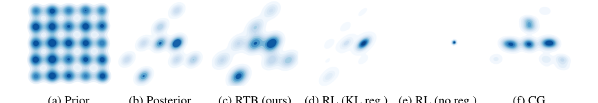Figure 1. Sampling densities learned by various posterior inference methods. The prior is a diffusion model sampling a mixture of 25 Gaussians (a) and the posterior is the product of the prior with a constraint that masks all but 9 of the modes (b). Our method (RTB) samples close to the true posterior (c). RL methods with tuned KL regularization yield inaccurate inference (d), while without KL regularization, they mode-collapse (e). A classifier guidance (CG) approximation (f) results in biased outcomes. For details, see §C 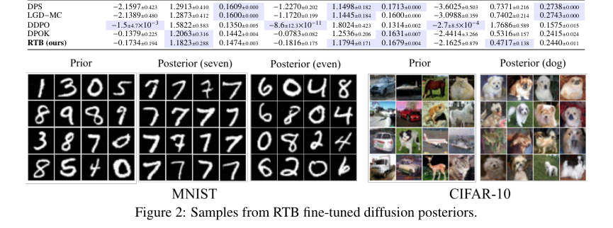Figure 2. Samples from RTB fine-tuned diffusion posteriors 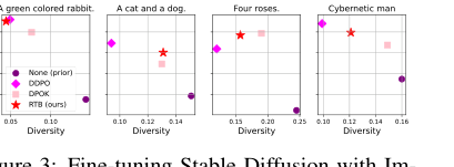Figure 4. Images generated from prior (top row), DPOK (middle row) and RTB (bottom row) for 4 different prompts. Images in the same column share the random DDIM seed. More images in §H.2 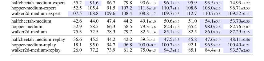Table 4. Average rewards of trained policies on D4RL locomotion tasks (mean±std over 5 random seeds). Following past work, numbers within 5% of maximum in every row are highlighted