Differentiated optimal control strategy of brucellosis in Ningxia, China: insights from a two-patch dynamical model

Background & Academic Lineage

The Origin & Academic Lineage

The problem addressed in this paper originates from the persistent and spatially heterogeneous nature of brucellosis, a zoonotic infectious disease, particularly in high-incidence regions like Ningxia, China. Historically, brucellosis has been a global concern, with significant prevalence in regions including the Mediterranean, Middle East, and parts of Asia, as noted in early literature [1]. In China, the disease experienced a notable resurgence from the mid-1990s, peaking in 2014, and its geographical spread expanded from traditional pastoral areas to agricultural and even southern coastal regions [3]. This expansion highlighted the disease's dual threat: causing substantial economic losses to the livestock industry due to animal infertility and reduced production [4, 5], while also posing a serious public health risk with hundreds of thousands of human cases reported annually worldwide [2].

The emergence of this specific problem stems from the observation that brucellosis transmission exhibits significant spatial-temporal heterogeneity and clustering [6, 7]. Factors like transregional livestock movement, especially from high-risk to low-risk areas [8], and environmental conditions such as air pressure and temperature [9], profoundly influence its spread. Previous epidemiological research primarily relied on statistical models for prediction. However, these models proved limited in capturing the intricate, dynamic interactions of the epidemic with human activities and the natural environment across different locations and over time. This fundamental limitation created a pressing need for a more sophisticated approach that could precisely identify high-risk areas and facilitate the allocation of differentiated resources for prevention and control. Dynamical modeling, therefore, became an essential tool to quantify the effects of this spatial heterogeneity and to formulate optimal, tailored prevention strategies [10-12]. The paper specifically focuses on Ningxia, a region with a severe brucellosis epidemic driven by B. melitensis in sheep [26], aiming to provide a quantitative basis for precise, differentiated control strategies given limited health resources.

Intuitive Domain Terms

• Brucellosis: Imagine a very persistent "animal flu" that can easily jump from infected animals (like sheep) to humans, causing long-term illness in both. For farmers, it's a double whammy: their animals get sick, leading to miscarriages and less milk/meat, and they themselves can catch it.
• Spatial-temporal heterogeneity: Think of a disease spreading not like a uniform fog, but more like a patchy, shifting storm. It's much worse in some towns than others, and its intensity changes with the seasons or over several years. This means the disease isn't everywhere at the same strength all the time.
• Patch model: Picture a map of a region divided into a few distinct zones or "neighborhoods." A patch model is like tracking how a disease spreads within each neighborhood and how it moves between them, acknowledging that each zone might have different conditions or risk levels.
• Basic reproduction number ($R_0$): This is like the "contagion score" for a disease. If one sick animal, on average, infects more than one other animal, the score is above 1, and the disease will likely spread. If it infects less than one, the score is below 1, and the disease will eventually die out.
• Optimal control strategy: Consider a general trying to win a war with limited soldiers and supplies. An optimal control strategy is the best possible battle plan that tells the general exactly when, where, and how much to deploy their resources (e.g., vaccines, movement restrictions) to achieve victory (minimize disease) most effectively.

Notation Table

Notation	Description

Problem Definition & Constraints

Core Problem Formulation & The Dilemma

The core problem addressed by this paper is the development of effective and differentiated optimal control strategies for brucellosis in Ningxia, China, a region characterized by a high incidence and significant spatial-temporal heterogeneity of the disease.

The input or current state is a complex epidemiological situation where brucellosis transmission exhibits distinct spatial-temporal patterns, leading to high-risk and low-risk areas (as illustrated in Figure 1). Health resources for prevention and control are limited, making uniform intervention strategies inefficient and often unfeasible. Furthermore, livestock movement between regions is a known driver of disease spread, complicating control efforts. Previous research, primarily relying on statistical models, has struggled to capture the intricate spatio-temporal dynamics and interactions with human activities and the natural environment. While vaccination is available and somewhat effective (e.g., M5 vaccine with ~65% efficacy), achieving uniform coverage across all regions is challenging due to resource scarcity.

The desired endpoint or goal state is to reduce the cumulative infected sheep population in both high-risk and low-risk patches by rationally allocating vaccination resources and implementing effective transportation supervision. This requires a quantitative framework to inform precise control strategies tailored to the specific risk levels of different areas.

The exact missing link or mathematical gap this paper attempts to bridge is the lack of a robust, spatially explicit dynamical model that integrates both spatial heterogeneity (two-patch system) and vaccination effects, coupled with an optimal control framework. Specifically, the paper aims to mathematically derive and evaluate optimal control solutions that account for differentiated interventions, moving beyond generic strategies to resource-efficient, targeted approaches.

The painful trade-off or dilemma that has trapped previous researchers, and which this paper seeks to navigate, is the challenge of achieving comprehensive disease control under severe resource limitations while simultaneously addressing the inherent spatial-temporal heterogeneity of brucellosis transmission. Often, improving control in one area or through one method (e.g., widespread vaccination) would demand exponentially more resources, which are simply not available. The dilemma is further exacerbated by migration patterns: while migration can increase brucellosis risk in low-risk patches, it can also have a "dilution effect" in high-risk areas (Remark 2, Page 11), meaning that simplistic, undifferentiated control measures might inadvertently worsen the situation in certain patches or misallocate precious resources. The authors aim to find a balance, ensuring that interventions are both effective and resource-prudent.

Constraints & Failure Modes

The problem of controlling brucellosis in Ningxia is made insanely difficult by several harsh, realistic constraints:

• Physical/Biological Constraints:

  • Zoonotic Nature and Transmission Dynamics: Brucellosis is a zoonotic disease primarily transmitted from infected animals (sheep) to humans, making control efforts complex as they involve both animal health and public health. The most pathogenic species in small ruminants, B. melitensis, is prevalent in Ningxia (Page 3).
  • Spatial-Temporal Heterogeneity: The incidence of brucellosis shows significant variation across space and time, necessitating a differentiated approach rather than a uniform one (Page 1, Abstract).
  • Livestock Migration: Transregional livestock movement is a major driver of disease spread (Page 2), making border control and transportation supervision critical but difficult to enforce perfectly.
  • Vaccination Efficacy: While vaccines exist, their effectiveness is not 100% (around 65% for M5 vaccine, Page 3), meaning vaccination alone cannot completely eradicate the disease.

• Computational/Mathematical Constraints:

  • Complex Epidemic Dynamics: The transmission dynamics of brucellosis involve intricate interactions between susceptible, infected, and vaccinated populations across different patches, which are challenging for simpler statistical models to capture effectively (Page 2).
  • Optimal Control Problem Complexity: Deriving optimal control solutions requires solving a system of differential equations for the state variables and associated costate variables, often involving non-linear functions and the application of Pontryagin's Maximum Principle (Section 4, Page 11). The control variables $u_i(t)$ are bounded within $[0, 1]$, representing the feasible range of intervention efforts.

• Data-Driven Constraints:

  • Data Scarcity for Sheep Infection: A significant constraint is the "lack of direct data on brucellosis infection in sheep herds" (Page 16). This forces the authors to estimate sheep infection rates indirectly from human brucellosis positivity rates using a linear regression model (Equation 5.1). This indirect estimation, despite a high $R^2$ value, introduces a potential "data bias" (Page 21).
  • Model Simplifications: The current model assumes uniform mixing of sheep within each patch and ignores the influence of population structure (e.g., age, breeding types) on disease spread (Page 21).
  • Deterministic Model Limitations: The deterministic nature of the model cannot fully capture random events, such as the stochastic migration of infected sheep, which can impact transmission (Page 21).

• Resource Constraints:

  • Limited Health Resources: The overarching constraint is the "limited health resources" available for brucellosis prevention and control (Page 1, Abstract; Page 3). This directly impacts the ability to implement widespread, uniform interventions.
  • Limited Immunization Resources: Specifically, limited resources for immunization make achieving uniform vaccination coverage across entire regions challenging (Page 3).
  • Uneven Resource Distribution: Health resources are "relatively unevenly distributed" (Page 20), further complicating equitable and effective control efforts.

Why This Approach

The Inevitability of the Choice

The adoption of a two-patch Susceptible-Infected-Vaccinated (SIV) sheep dynamical model, coupled with optimal control theory, was not merely a choice but an inevitable necessity given the inherent complexities of brucellosis transmission in Ningxia. The authors explicitly recognized the limitations of traditional "SOTA" methods, particularly statistical models, which form the previous gold standard in many epidemiological studies. As stated in the introduction, "Existing research mainly focuses on using statistical models for epidemic prediction, but these models have limitations in handling the complex dynamics of epidemic transmission and are difficult to effectively capture the spatio-temporal interactions with human activities and the natural environment." This realization marked the exact moment when a departure from purely statistical approaches became imperative.

Statistical models, while useful for prediction, often struggle to mechanistically represent the dynamic interplay of disease spread, population movement, and intervention effects over time and space. Brucellosis in Ningxia exhibits significant spatial-temporal heterogeneity, meaning its prevalence varies considerably across different geographical areas and changes over time. To charaterize these complex dynamics and, crucially, to formulate optimal and differentiated control strategies, a dynamic modeling framework was the only viable path. A compartmental model like SIV allows for the explicit representation of population states (susceptible, infected, vaccinated) and the transitions between them, providing a mechanistic understanding that statistical correlations alone cannot offer.

Comparative Superiority

This two-patch SIV dynamical model offers qualitative superiority over previous approaches primarily through its structural ability to capture and optimize complex, interacting epidemiological processes. Unlike simpler statistical models, it doesn't just predict outcomes; it provides a framework to understand why and how the disease spreads and what interventions are most effective.

1. Spatio-temporal Heterogeneity: The division into "high-risk" and "low-risk" patches, as depicted in Figure 1, is a fundamental structural advantage. This allows the model to account for varying disease dynamics and intervention needs in different geographical areas, which is critical for a region like Ningxia.
2. Dynamic Interactions and Migration: The model explicitly incorporates migration rates ($a_{12}, a_{21}, b_{12}, b_{21}, c_{12}, c_{21}$) between patches for susceptible, infected, and vaccinated sheep. This is a crucial structural improvement over single-patch models or statistical methods that might overlook the impact of cross-regional movement on disease spread. As Remark 2 highlights, ignoring migration can "overestimate or underestimate the basic reproduction number of different patches."
3. Optimal Control Framework: The integration of Pontryagin's Maximum Principle to derive optimal control solutions ($u_1$ to $u_6$) is a significant qualitative leap. This allows for the quantitative evaluation of different intervention strategies (personal protection, vaccination, migration supervision) and their optimal allocation over time, under the constraint of limited resourse. This goes beyond simple performance metrics by providing actionable, time-dependent strategies, rather than just a static assessment of effectiveness.
4. Mechanistic Understanding: The SIV structure provides a clear, interpretable mechanism for disease transmission, recovery, and immunity, which is more robust for policy formulation than black-box predictive models. It allows for the calculation of key epidemiological parameters like the basic reproduction number ($R_0$), offering insights into disease persistence and stability.

The paper does not discuss high-dimensional noise handling or memory complexity, as these are not the primary comparative axes for this type of epidemiological modeling against its relevant alternatives (statistical models, simpler ODE models). Its superiority lies in its ability to model complex dynamic systems with spatial interactions and optimize interventions within that system.

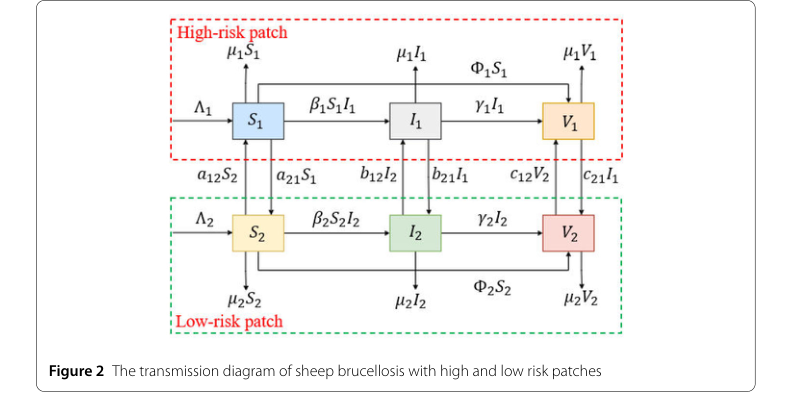Figure 2. The transmission diagram of sheep brucellosis with high and low risk patches

Alignment with Constraints

The chosen two-patch SIV dynamical model with optimal control theory perfectly aligns with the problem's harsh requirements, forming a robust "marriage" between the problem and its solution.

1. Spatial Heterogeneity: The problem explicitly identifies Ningxia as a high-incidence region with "significant spatial-temporal heterogeneity." The two-patch structure (high-risk and low-risk) directly addresses this by allowing for distinct parameters and dynamics in each area, as well as interactions between them.
2. Limited Health Resources: A core constraint is the need to achieve prevention and control objectives "under limited health resources." The optimal control framework is inherently designed for this. By defining an objective function (4.2) that minimizes both the cumulative infected population and the costs associated with control efforts, the model provides a strategy for the most efficient allocation of scarce resources.
3. Differentiated Control Strategies: The prompt for "differentiated control strategies" is met by the model's ability to define six distinct control functions ($u_1$ to $u_6$) for various interventions (personal protection, vaccination, migration supervision) across both patches. The optimal control solution then determines the ideal time-varying application of these controls, leading to strategies tailored to each patch's specific risk profile.
4. Quantifying Intervention Effects: The problem necessitates quantifying the preventive effect of vaccination and transportation supervision. The SIV model explicitly includes vaccination compartments ($V_i$) and control variables ($u_2, u_5$ for vaccination; $u_3, u_6$ for migration supervision) that directly modulate these processes, allowing for their quantitative assessment within the optimal control framework.

Rejection of Alternatives

The paper implicitly and explicitly rejects several alternative approaches based on their inability to address the core problem characteristics.

1. Statistical Models: The most direct rejection is of "statistical models for epidemic prediction." The authors state these models "have limitations in handling the complex dynamics of epidemic transmission and are difficult to effectively capture the spatio-temporal interactions with human activities and the natural environment." This highlights their insufficiency for a problem requiring a mechanistic understanding of dynamic spread and optimal intervention.
2. Single-Patch Dynamical Models: While not explicitly named, the paper's emphasis on "spatial-temporal heterogeneity" and the construction of a "two-patch" model inherently rejects single-patch models. Remark 2 further solidifies this by explaining that ignoring migration in single-patch models "may overestimate or underestimate the basic reproduction number of different patches," leading to inaccurate assessments and suboptimal strategies. The need for "cross-regional collaborative combined control strategies" also necessitates a multi-patch approach.
3. Deterministic Models for Stochastic Events: In the "Limitations" section (Section 6), the authors acknowledge that their deterministic model cannot describe "random events such as the random migration of infected sheep." This implies a rejection of purely deterministic models for scenarios where stochasticity plays a significant role, suggesting future work might incorporate stochastic processes like the Ornstein-Uhlenbeck process.
4. Generic Machine Learning Models (e.g., GANs, Diffusion, Transformers): The prompt mentions these as "SOTA" methods. However, in the context of epidemiological modeling for optimal control, these are not directly applicable alternatives. They are designed for different tasks (e.g., image generation, natural language processing) and lack the mechanistic structure required to model disease transmission dynamics and derive interpretable control policies. The paper does not mention or reject these specific types of models, as they fall outside the scope of traditional epidemiological modeling comparisons. The relevant alternatives are within the domain of epidemiological and mathematical modeling.

Mathematical & Logical Mechanism

The Master Equation

The absolute core of this paper's mathematical engine is the objective function, which quantifies the overall cost associated with the brucellosis epidemic and its control efforts. The goal is to minimize this function over a specified time horizon $T$. It is expressed as:

$$ J = \int_0^T \left[ A_1I_1(t) + A_2I_2(t) + \frac{1}{2} \sum_{i=1}^6 B_i u_i^2(t) \right] dt $$

This equation, coupled with the system of ordinary differential equations (ODEs) that describe the two-patch SIV (Susceptible-Infected-Vaccinated) model under control, forms the complete optimal control problem. The ODEs, which define the dynamics of the sheep populations, are implicitly part of this mechanism as they dictate how $I_1(t)$, $I_2(t)$, and the effects of $u_i(t)$ evolve over time.

Term-by-Term Autopsy

Let's dissect the master equation and its components, along with the control variables that influence the underlying dynamical system:

• $J$:

  • Mathematical Definition: A scalar value representing the total accumulated cost.
  • Physical/Logical Role: This is the quantity the authors aim to minimize. It serves as a comprehensive measure of the epidemic's burden (due to infected populations) and the resources expended on control strategies over the entire intervention period.
  • Why integral: The system's dynamics are continuous over time, so an integral is used to sum up the instantaneous costs continuously from the initial time $t=0$ to the final time $t=T$. This provides a total, cumulative cost rather than a snapshot.

• $\int_0^T \dots dt$:

  • Mathematical Definition: A definite integral over the time interval $[0, T]$.
  • Physical/Logical Role: This operator accumulates the instantaneous value of the integrand (the cost function at a given moment) over the entire duration of the control intervention.
  • Why integral: As the state variables and control actions are considered continuous functions of time, an integral is the natural mathematical tool to sum their effects over a continuous period.

• $A_1I_1(t)$:

  • Mathematical Definition: The product of a positive weight coefficient $A_1$ and the number of infected sheep $I_1$ in patch 1 at time $t$.
  • Physical/Logical Role: This term represents the instantaneous cost or burden associated with the infected population in the high-risk patch (patch 1). A higher $A_1$ signifies a greater priority or penalty for infections in this patch, driving the optimization to reduce $I_1$.
  • Why addition: This term is added to the total cost because it represents an undesirable outcome (infections) that contributes to the overall burden.

• $A_2I_2(t)$:

  • Mathematical Definition: The product of a positive weight coefficient $A_2$ and the number of infected sheep $I_2$ in patch 2 at time $t$.
  • Physical/Logical Role: Similar to $A_1I_1(t)$, this term represents the instantaneous cost associated with the infected population in the low-risk patch (patch 2). $A_2$ weights the importance of reducing $I_2$.
  • Why addition: It's an additive component to the total cost, reflecting another source of burden.

• $A_1, A_2$:

  • Mathematical Definition: Positive constant coefficients.
  • Physical/Logical Role: These are "tuning parameters" that allow the modelers to assign relative importance to reducing infected populations in each patch. For instance, if $A_1 > A_2$, it implies that reducing infections in patch 1 is considered more critical or costly than in patch 2.
  • Why coefficients: They provide flexibility in balancing the objectives of the control strategy.

• $I_1(t), I_2(t)$:

  • Mathematical Definition: State variables representing the number of infected sheep in patch 1 and patch 2, respectively, at time $t$. These are non-negative real numbers.
  • Physical/Logical Role: These are the primary targets of the control strategy. Minimizing $J$ directly aims to reduce these populations. Their dynamics are governed by the system of ODEs (4.1).

• $\frac{1}{2} \sum_{i=1}^6 B_i u_i^2(t)$:

  • Mathematical Definition: Half the sum of quadratic terms for each of the six control variables, weighted by positive coefficients $B_i$.
  • Physical/Logical Role: This term represents the instantaneous cost of implementing the control strategies. The quadratic form ($u_i^2$) means that applying stronger control efforts incurs a disproportionately higher cost, discouraging excessive or unrealistic interventions. This also ensures the cost is always non-negative.
  • Why summation: There are six distinct control measures, and their individual costs are aggregated to form the total control cost.
  • Why quadratic ($u_i^2$): The quadratic form is a standard choice in optimal control for several reasons: it ensures the cost is always positive, it penalizes larger control efforts more heavily (making the optimization "work harder" for diminishing returns), and it often contributes to the convexity of the objective function, which simplifies finding a unique optimal solution.

• $B_i$:

  • Mathematical Definition: Positive constant coefficients for each control variable $u_i$.
  • Physical/Logical Role: These coefficients determine the relative cost of applying each specific control measure. A higher $B_i$ means that control $u_i$ is more expensive or resource-intensive to implement.
  • Why coefficients: They allow for fine-tuning the balance between reducing infections and the cost of specific interventions.

• $u_i(t)$ ($u_1, \dots, u_6$):

  • Mathematical Definition: Time-dependent control functions, constrained to be within $[0, 1]$.
  • Physical/Logical Role: These are the decision variables that the optimization process seeks to determine. They represent the intensity or effectiveness of different control measures:
    • $u_1(t)$: Control effect of personal protection behaviors in patch 1. In the ODEs, it reduces the effective transmission rate $(1-u_1)\beta_1S_1I_1$.
    • $u_2(t)$: Control effect of vaccination in patch 1. In the ODEs, it moves susceptible sheep $S_1$ to the vaccinated class $V_1$ at a rate $u_2S_1$.
    • $u_3(t)$: Control effect on migration from patch 1 to patch 2. In the ODEs, it reduces the outflow of $S_1, I_1, V_1$ from patch 1 to patch 2.
    • $u_4(t)$: Control effect of personal protection behaviors in patch 2. Similar to $u_1$, it reduces the effective transmission rate $(1-u_4)\beta_2S_2I_2$.
    • $u_5(t)$: Control effect of vaccination in patch 2. Similar to $u_2$, it moves susceptible sheep $S_2$ to $V_2$ at a rate $u_5S_2$.
    • $u_6(t)$: Control effect on migration from patch 2 to patch 1. Similar to $u_3$, it reduces the outflow of $S_2, I_2, V_2$ from patch 2 to patch 1.

Step-by-Step Flow

Imagine the system as a complex, interconnected assembly line where sheep populations move between compartments and patches, influenced by control levers.

1. Initial State Setup: The process begins with a defined initial number of susceptible ($S_1(0), S_2(0)$), infected ($I_1(0), I_2(0)$), and vaccinated ($V_1(0), V_2(0)$) sheep in both the high-risk (patch 1) and low-risk (patch 2) areas. These initial conditions set the starting point for the epidemic's trajectory.

2. Control Lever Adjustment: At any given moment $t$, the six control levers ($u_1(t)$ through $u_6(t)$) are set to specific values, representing the intensity of intervention. For example, if $u_2(t)$ is high, it means a strong vaccination campaign is active in patch 1. If $u_3(t)$ is high, it implies strict measures are in place to restrict sheep movement from patch 1 to patch 2.

3. Population Dynamics Simulation: These control settings directly impact the rates of change for each sheep population in both patches, as described by the system of six coupled ODEs (4.1).

   • Infection Reduction: Controls $u_1$ and $u_4$ act like "shields," reducing the rate at which susceptible sheep become infected in their respective patches.
   • Vaccination Drive: Controls $u_2$ and $u_5$ act as "conveyors," moving susceptible sheep into the vaccinated compartment, making them immune.
   • Migration Management: Controls $u_3$ and $u_6$ act as "gatekeepers," regulating the flow of susceptible, infected, and vaccinated sheep between the two patches. For instance, $u_3$ reduces sheep leaving patch 1 for patch 2, while $u_6$ reduces sheep leaving patch 2 for patch 1.
   • Natural Processes: Alongside controls, natural birth rates ($A_1, A_2$), natural death rates ($\mu_1, \mu_2$), and recovery rates ($\gamma_1, \gamma_2$) continuously influence the population sizes.

4. Instantaneous Cost Calculation: As the populations evolve, at each moment $t$, two types of costs are calculated:

   • Epidemic Burden: The current number of infected sheep in each patch ($I_1(t)$ and $I_2(t)$) contributes to the cost, weighted by $A_1$ and $A_2$. This is like a "meter" measuring the ongoing impact of the disease.
   • Intervention Expense: The current settings of the control levers ($u_i(t)$) also incur a cost, weighted by $B_i$ and squared. This is like a "fuel gauge" showing how much resource is being consumed by the interventions.

5. Total Cost Accumulation: These instantaneous costs are continuously added up over the entire intervention period (from $t=0$ to $t=T$) by the integral operator, resulting in the single total cost value $J$.

6. Optimization Loop (Conceptual): The entire "assembly line" is run repeatedly with different settings of the control levers (the $u_i(t)$ functions). The goal is to find the specific set of control functions that makes the final accumulated cost $J$ as small as possible. This search for the optimal control strategy is the essence of the optimization dynamics.

Optimization Dynamics

The mechanism learns, updates, and converges through the application of Pontryagin's Maximum Principle, a fundamental tool in optimal control theory. This principle transforms the original problem of minimizing the objective function $J$ subject to the system's dynamics into a more tractable problem involving a Hamitonian function.

1. The Hamiltonian Formulation: The first step is to construct the Hamiltonian function, $H$, as defined in equation (4.10). This function combines the objective function's integrand (the instantaneous cost) with the right-hand sides of the state equations (the population dynamics), each weighted by a corresponding "costate variable" ($\lambda_{ij}$). The costate variables essentially represent the shadow price or marginal contribution of each state variable to the overall objective function.

2. Costate Equations (Adjoint System): To find the optimal path, we need to understand how the costate variables evolve. This is done by deriving a system of differential equations for the costate variables (equation (4.11)). These equations are obtained by taking the partial derivative of the Hamiltonian with respect to each state variable. Crucially, unlike the state equations which run forward in time, the costate equations are typically solved backward in time, starting from a terminal condition (here, $\lambda_{ij}(T) = 0$, meaning there's no future cost associated with the state at the end of the control period).

3. Optimality Conditions for Controls: The core of finding the optimal controls lies in minimizing the Hamiltonian with respect to the control variables at each point in time. This is achieved by setting the partial derivative of the Hamiltonian with respect to each control variable to zero ($\frac{\partial H}{\partial u_i} = 0$). This yields explicit expressions for the optimal controls $u_i^*$ (equation (4.12)), which are functions of both the state variables ($S_i, I_i, V_i$) and the costate variables ($\lambda_{ij}$). These expressions are then typically "clipped" or projected onto the feasible control set, which is $[0, 1]$ for each $u_i$.

4. Iterative Solution (Forward-Backward Sweep): The state equations (forward in time) and costate equations (backward in time) are coupled through the Hamiltonian and the optimality conditions for the controls. This forms a two-point boundary value problem that cannot be solved directly. Instead, an iterative numerical method, often called a forward-backward sweep, is employed:

   • Initial Guess: An initial guess for the control functions $u_i(t)$ over the entire time horizon $[0, T]$ is made (e.g., all zeros or random values).
   • Forward Sweep: Using the current guess for the controls, the state equations (4.1) are integrated forward in time from $t=0$ to $t=T$ with their initial conditions. This yields a trajectory for all population sizes ($S_i(t), I_i(t), V_i(t)$).
   • Backward Sweep: Using the state trajectories obtained from the forward sweep, the costate equations (4.11) are integrated backward in time from $t=T$ to $t=0$ with their terminal conditions. This yields a trajectory for all costate variables ($\lambda_{ij}(t)$).
   • Control Update: With the updated state and costate trajectories, the optimality conditions (4.12) are used to calculate a new, improved set of control functions $u_i(t)$.
   • Convergence Check: Steps 2-4 are repeated. The process continues until the control functions, state variables, and costate variables converge, meaning the change between successive iterations falls below a predefined tolerance. This iterative refinement allows the mechanism to "learn" the optimal control strategy.

5. Loss Landscape and Gradients: The objective function $J$ defines a multi-dimensional "loss landscape." The optimization process essentially navigates this landscape. The costate variables can be thought of as generalized gradients, indicating the direction of steepest ascent (or descent for minimization) in this landscape. The quadratic terms in the objective function for the controls ($B_i u_i^2$) contribute to making this landscape convex, which is a desirable property as it generally guarantees that the iterative process will converge to a unique global minimum, rather than getting stuck in local minima. The iterative updates adjust the controls in a way that reduces the total cost, effectively moving down the loss landscape until a minimum is reached, representing the optimal balance between reducing infections and minimizing intervention costs. This iterative process allows the model to find the most effective and efficient control strategy over time. The careful balance of costs and benefits in the objective function shapes this landscape, guiding the convergeance towards a practical solution.

Results, Limitations & Conclusion

Experimental Design & Baselines

To rigorously test their mathematical claims, the authors embarked on a comprehensive experimental validation process. The core of their approach involved calibrating their two-patch SIV sheep brucellosis model (model 2.1) using real-world surveillance data from Ningxia, China, spanning from 2010 to 2019. A critical challenge was the absence of direct historical data on infected sheep populations. To overcome this, they ingeniously employed a linear regression analysis to estimate the sheep brucellosis positivity rate ($x$) from the human brucellosis positivity rate ($y$) (per 100,000 population) observed between 2022 and 2024 in Ningxia. This yielded a robust linear regression equation: $y = 0.0044x + 2.5822 + \epsilon$, where $\epsilon \sim N(0,0.1544)$, boasting an impressive coefficient of determination $R^2 = 0.9962$ (as illustrated in Figure 4a). This relationship allowed them to estimate the historical newly infected shep cases in both high-risk and low-risk patches from 2010 to 2019.

With this estimated data, the model (2.1) was then calibrated using the Least Squares method. The initial conditions for the model were set as $S_1(0) = 1,898,000$, $I_1(0) = 42,724$, $V_1(0) = 0$ for the high-risk patch, and $S_2(0) = 2,353,000$, $I_2(0) = 9091$, $V_2(0) = 0$ for the low-risk patch. The various parameters, including birth rates, transmission coefficients, vaccination rates, natural death rates, recovery rates, and migration rates between patches, were either fitted from the data, calculated, or sourced from existing literature, as detailed in Table 1.

The "victims" or baseline models against which the proposed optimal control strategies were compared were essentially the scenarios where no control interventions were applied. This "without control" state served as the benchmark to definitively demonstrate the efficacy of their core mechanism – the differentiated optimal control strategies derived from Pontryagin's Maximum Principle. By comparing the cumulative change in infected sheep cases under various control combinations against this baseline, they sought undeniable evidence that their proposed interventions could significantly reduce disease prevalence.

What the Evidence Proves

The evidence presented in the paper strongly supports the efficacy of the proposed differentiated optimal control strategies. First, the model calibration proved highly successful; the fitted results for newly infected sheep cases in both high-risk and low-risk patches (Figures 4b and 4c) showed excellent consistency with the estimated historical data. This consistency provides a solid foundation for the model's predictive capabilities and the subsequent optimal control analysis.

The numerical simulations, particularly those depicted in Figure 5, clearly demonstrate the existence and dynamic behavior of the optimal control solutions over time. The core mechanism of their approach, which is the application of optimal control theory to a two-patch SIV model, is shown to work in reality by identifying specific intervention profiles:
- Vaccination in high-risk patches ($u_2$): This control variable consistently maintained its maximum value throughout the intervention period, underscoring its critical role in brucellosis control within high-risk areas.
- Vaccination in low-risk patches ($u_5$): This intervention showed substantial influence initially but then declined to zero in later stages, suggesting that sustained high vaccination rates might not be necessary in low-risk areas over the long term.
- Restricting transport from low-risk to high-risk patches ($u_6$): This control remained at relatively high levels initially but then decreased, indicating its importance in preventing disease reintroduction into high-risk areas.
- Health education in high-risk patches ($u_1$) and transport from high-risk to low-risk patches ($u_3$): These controls increased in later stages, implying that enhanced health education and a moderate increase in sheep transport from high-risk to low-risk areas could be beneficial in the long run.
- Health education in low-risk patches ($u_4$): This control remained at low levels, suggesting a less significant impact on disease control in these areas.

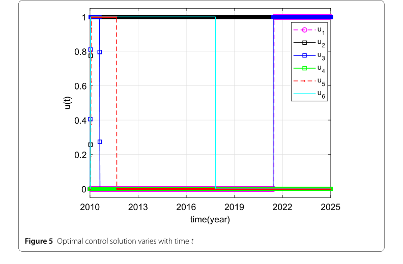Figure 5. Optimal control solution varies with time t

Furthermore, the analysis of local control strategies (Figure 7) revealed that while individual interventions like $u_2$ (vaccination in high-risk) and $u_3$ (transport from high-risk to low-risk) could significantly reduce infections in high-risk patches, and $u_5$ (vaccination in low-risk) and $u_6$ (restricting transport from low-risk to high-risk) were effective in low-risk patches, local strategies alone might not be sufficent to achieve the overall control objective for brucellosis in Ningxia.

The definitive evidence for their core mechanism's effectiveness came from the evaluation of cross-patch combined control strategies (Figure 8). The strategy $S_{12}$ (combining $u_2$, $u_3$, and $u_5$) emerged as the most effective for the high-risk patch, leading to the largest cumulative decrease in infected sheep. For the low-risk patch, strategy $S_{10}$ (combining $u_2$, $u_5$, and $u_6$) generated the largest positive cumulative change, indicating its superior performance in reducing infections. This undeniably proves that a differentiated, combined approach, tailored to the specific risk level of each patch, is crucial for effective brucellosis control.

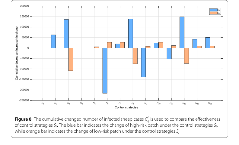Figure 8. The cumulative changed number of infected sheep cases CI ij is used to compare the effectiveness of control strategies Sj. The blue bar indicates the change of high-risk patch under the control strategies Sj, while orange bar indicates the change of low-risk patch under the control strategies Sj

Limitations & Future Directions

While this study offers valuable insights and a robust framework for brucellosis control, it's important to acknowledge its inherent limitations, which naturally open avenues for future research.

Firstly, a significant limitation stems from the indirect estimation of sheep brucellosis infection rates. Due to the lack of direct historical data on infected sheep herds in Ningxia, the authors had to infer these rates from human brucellosis incidence data using a linear regression model. Although the regression showed a high $R^2$ value, this indirect estimation method may introduce data biass [47]. This reliance on proxy data could potentially affect the precision of the model's calibration and, consequently, the derived optimal control strategies.

Secondly, the current model assumes a uniform mixing of sheep populations within each patch, neglecting the intricate influence of population structure. Factors such as age, different breeding types, and specific cross-patch interactions that go beyond simple migration rates are not explicitly accounted for [48]. In reality, these structural elements can significantly alter disease transmission dynamics, meaning the model might not fully capture the complexity of brucellosis spread in diverse livestock populations.

Thirdly, the use of a deterministic model inherently limits its ability to describe random events. Phenomena such as the stochastic migration of infected sheep, which can have a considerable impact on disease transmission, cannot be captured by the current framework [49]. Real-world epidemics are often influenced by unpredictable events, and a deterministic approach might oversimplify these crucial aspects.

Looking ahead, these limitations naturally suggest several promising directions for further development and evolution of these findings:

1. Incorporating Population Structure: Future research should aim to integrate more detailed population structures into the sheep brucellosis model. This could involve developing an age-structured model or differentiating between various breeding types (e.g., dairy sheep vs. meat sheep) to better understand their specific roles in transmission. Such an approach would provide a more nuanced understanding of how different sub-populations contribute to the overall epidemic and how interventions can be tailored more precisely.

2. Modeling Stochasticity: To address the deterministic nature of the current model, future work could incorporate stochastic processes. Specifically, employing an Ornstein-Uhlenbeck process to depict environmental stochasticity or random migration events would be highly valuable. This would allow for a more realistic assessment of how randomness impacts transmission dynamics and the robustness of control strategies, potentially leading to more resilient intervention plans.

3. Direct Data Collection and Validation: A long-term goal should be to facilitate and utilize direct, comprehensive surveillance data on brucellosis infection in sheep herds. This would eliminate the need for indirect estimation, significantly improving the accuracy of model calibration and validation. Collaborative efforts between public health agencies, veterinary services, and researchers could be instrumental in establishing such data collection systems.

4. Economic Cost-Benefit Analysis: While the current study focuses on optimal control to minimize infected populations, future research could expand to include a detailed economic cost-benefit analysis of different control strategies. This would provide policymakers with a more holistic view, balancing disease reduction with resource allocation efficiency, especially given limited health resources.

By addressing these points, the findings can be further refined, leading to even more precise, robust, and practically applicable brucellosis control strategies in regions like Ningxia and beyond.

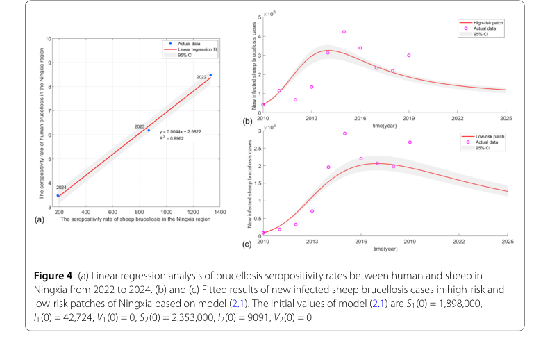Figure 4. (a) Linear regression analysis of brucellosis seropositivity rates between human and sheep in Ningxia from 2022 to 2024. (b) and (c) Fitted results of new infected sheep brucellosis cases in high-risk and low-risk patches of Ningxia based on model (2.1). The initial values of model (2.1) are S1(0) = 1,898,000, I1(0) = 42,724, V1(0) = 0, S2(0) = 2,353,000, I2(0) = 9091, V2(0) = 0