Accelerating atomic fine structure determination with graph reinforcement learning

Background & Academic Lineage

The Origin & Academic Lineage

The problem addressed in this paper, known as "term analysis," originates from the fundamental need to understand the atomic structure of elements. Specifically, it involves extracting the energies and total electron angular momenta ($J$) of energy levels from observed atomic spectra, and assigning appropriate term symbols to these levels. This field of study is crucial because the resulting atomic data, such as energy levels and transition wavenumbers, are essential for a wide array of applications. These include plasma diagnostics, the lighting and metal industries, magnetic confinement fusion research, nuclear research, medical isotope production, and astronomy, particularly in understanding the origin of heavy elements from events like neutron star mergers.

Historically, the process of term analysis has been a sequential, complex decision-making task demanding both deep atomic spectroscopy expertise and extensive human labor. Since the introduction of Fourier transform (FT) spectroscopic term analyses in the 1970s, its application has largely been confined to the iron-group elements (those with atomic numbers $Z$ between 23 and 28). The challenge stems from the immense number of observable spectral lines (often tens of thousands for each element) that represent energy differences between levels, making the determination of individual energy levels a daunting task, guided only by less accurate theoretical predictions.

The fundamental limitation, or "pain point," of previous approaches is their extreme inefficiency and reliance on human experts. While the initial steps of spectrum measurement and theoretical calculations for a single atomic species can be completed in weeks, the subsequent term analysis—the crucial step of identifying energy levels from the observed data—can take months to years. This manual, labor-intensive process has become a major bottleneck, preventing the rapid generation of atomic data needed to meet growing demands across various scientific and industrial fields. Furthermore, existing ab initio (first-principles) calculations are often only accurate to a few percent, which is insufficient for applications requiring high spectral resolution. Term analyses, despite their human cost, offer orders-of-magnitude higher accuracies and provide reliable constraints for theoretical models. This inefficiency and the inability of theoretical methods alone to provide sufficient accuracy are the primary motivations for the authors to develop an automated, artificial intelligence-driven solution.

Intuitive Domain Terms

1. Atomic Fine Structure Determination / Term Analysis: Imagine you have a complex musical instrument, like a grand piano, but you can only hear the notes it plays, not see the keys or how they're arranged. "Atomic fine structure determination" is like figuring out the exact position and identity of every single key on that piano, and how they relate to each other, just by listening to the melodies. It's the process of mapping observed spectral "notes" back to the fundamental "keys" (energy levels) of an atom.

2. Spectral Line / Wavenumber ($\sigma$): Continuing the piano analogy, a "spectral line" is like a single, distinct note you hear. When an electron in an atom jumps from a higher energy level to a lower one, it emits light at a very specific "pitch." The "wavenumber" ($\sigma$) is the precise measurement of that pitch, telling us exactly how much energy was released in that electron jump. It's a direct measure of the energy difference between two atomic states.

3. Markov Decision Process (MDP): Think of an MDP as a treasure hunt game. You (the "agent") are in a certain location (the "state"), and you have several choices of paths to take (the "actions"). Each path you choose might lead you to a new location (a new state) and give you some gold (a "reward"). The goal of the game is to find a strategy (a "policy") that maximizes the total amount of gold you collect over the entire hunt, even if some paths have immediate small rewards but lead to dead ends later.

4. Reinforcement Learning (RL): This is like teaching a robot to play the treasure hunt game without giving it explicit instructions. Instead, you let the robot try different paths. When it finds gold, you tell it "good job!" (a positive reward). When it hits a dead end, you tell it "not so good" (a negative reward). Over many attempts, the robot learns through trial and error which actions in which states lead to the most gold, eventually becoming an expert treasure hunter.

5. Graph Neural Networks (GNNs): Consider a vast network of interconnected cities, where each city has unique characteristics (like population, industry) and each road connecting them has properties (like length, traffic). A GNN is a special type of artificial intelligence designed to understand and learn from the relationships and features within such a network. It helps the AI "see" the overall structure and local connections, allowing it to make informed decisions about the cities and roads, much like how it helps analyze the complex web of atomic energy levels and spectral lines.

Notation Table

Notation	Description
$J$	Total electron angular momentum
$Z$	Atomic number
$\sigma$	Wavenumber
$\sigma_{obs}$	Observed wavenumber
$\delta\sigma_{obs}$	Standard wavenumber uncertainty
$I_{obs}$	Relative intensity
$S/N_{obs}$	Signal-to-noise ratio
$E_{obs}$	Observed energy of an atomic level
$E_{calc}$	Theoretical energy of an atomic level
$\Delta E$	Theoretical uncertainty in energy level
$\Delta I$	Theoretical uncertainty in line intensity
$E_u$	Upper energy level
$E_l$	Lower energy level
$E_0$	Ground energy level (fixed at zero)
$s_t$	State at time $t$ in an MDP
$a_t$	Action taken at time $t$ in an MDP
$r_t$	Reward received at time $t$
$G_t$	Cumulative discounted reward from time $t$
$\gamma$	Discount factor
$H$	Finite horizon (episode length) in an MDP
$Q(s, a)$	Q-value (expected cumulative reward for taking action $a$ in state $s$)
$Q_{\theta}$	Online Q-network with parameters $\theta$
$Q_{\bar{\theta}}$	Target Q-network with parameters $\bar{\theta}$
$L$	Loss function
$TD[n]$	n-step Temporal Difference error
$r^{[n]}$	n-step return
$w_m$	Weight for line $m$ in least-squares optimization
$S_{mn}$	Coefficient matrix relating energy levels to line $m$
$M$	Total number of known lines
$N$	Total number of known levels
$D$	Preference score for an action $a^{(2)}$
$h_v$	Node embedding vector for level $v$
$S_{agg}$	Global graph state embedding vector
$V(s)$	State-value function
$A(s, a)$	Advantage function
MLP	Multi-Layer Perceptron
GNN	Graph Neural Network
$N_c$	Number of correctly determined energy levels
$R_{max}$	Maximum cumulative reward
Acc.	Accuracy of determined levels
PER	Prioritized Experience Replay
MCTS	Monte-Carlo Tree Search
UCT	Upper Confidence Bound for Trees

Problem Definition & Constraints

Core Problem Formulation & The Dilemma

The core problem addressed by this paper is the acceleration of atomic fine structure determination. This is a critical task in atomic spectroscopy, providing fundamental data for various scientific and industrial applications, from plasma diagnostics to astrophysics.

The starting point (Input/Current State) for this analysis is a collection of observed atomic spectra, which are preprocessed into a "line list." This line list contains approximately $10^4$ observable spectral lines for a given atomic species, each characterized by its observed wavenumber ($\sigma_{obs}$), standard wavenumber uncertainty ($\delta\sigma_{obs}$), relative intensity ($I_{obs}$), and signal-to-noise ratio ($S/N_{obs}$). Additionally, the current state includes a graph representation of known (empirically determined) energy levels and transitions, alongside theoretically predicted levels and lines. These known levels are typically connected, with their observed energies ($E_{obs}$) relative to a fixed zero energy ground level.

The desired endpoint (Output/Goal State) is to accurately determine the observed energies ($E_{obs}$) for unknown atomic energy levels and to classify spectral lines that best match theoretical predictions within experimental uncertainties. This involves expanding the subgraph of known levels by identifying and matching at least two observed spectral lines from the line list to corresponding edges connecting an unknown level to known levels, thereby determining the unknown level's energy.

The exact missing link or mathematical gap that this paper attempts to bridge lies in the transition from raw spectral line data and less accurate theoretical predictions to precise, empirically validated atomic energy levels. Historically, this process, known as "term analysis," has been a sequential, complex decision-making task requiring extensive human labor and atomic spectroscopy expertise, often taking months to years for a single atomic species. The mathematical gap is the lack of an automated, scalable, and accurate method to infer these energy levels from the vast number of observed spectral line differences, guided by theoretical but often imprecise calculations. The paper frames this as a Markov Decision Process (MDP) to be solved by graph reinforcement learning (GRL).

The painful trade-off or dilemma that has trapped previous researchers is the stark choice between accuracy and efficiency. While human-driven term analysis yields high accuracy (orders of magnitude higher than ab initio calculations) and reliable theoretical constraints, it is excruciatingly slow and labor-intensive, struggling to meet the growing demand for atomic data. Conversely, ab initio theoretical calculations are fast but typically only accurate to a few percent, which is insufficient for applications requiring higher spectral resolutions. The dilemma is that improving the speed of analysis traditionally meant sacrificing the necessary precision, or vice versa. This paper seeks to partially automate the process, aiming to achieve human-level accuracy at a significantly accelerated pace, thereby closing the gap between data demand and analysis capacity.

Constraints & Failure Modes

The problem of accelerating atomic fine structure determination is insanely difficult due to several harsh, realistic constraints:

• Physical & Domain-Specific Constraints:

  • Data Volume and Complexity: For each low-ionization open d- and f-subshell atomic species, determining around $10^3$ fine structure energy levels involves analyzing approximately $10^4$ observable spectral lines. The primary challenge is extracting precise energy levels from an "immense number of observed energy differences" (Section 1, p.3).
  • Inaccurate Theoretical Guidance: Existing theoretical predictions are often "less accurate" (Section 1, p.3), providing only a rough guide rather than precise values. Ab initio calculations are typically accurate only to a few percent, which is insufficient for many applications.
  • Ambiguity and Uncertainty: Determined energy levels often have "ambiguous values" (Section 2.5, p.5). Human experts must weigh agreement between observed and theoretical line intensities and the consistency of repeated $E_{obs}$ values within wavenumber uncertainties. This judgment is complicated by "uncertainties in transition probabilities and errors in spectral line fitting, especially for widespread weak and/or blended lines" (Section 2.5, p.6).
  • Limited Usable Transitions: Only electric dipole fine structure transitions are considered, as "higher order multipole transitions are rarely observed in the laboratory spectra" (Section 2.2, p.4), limiting the available data for analysis.
  • Outliers and Noise: The presence of "outlier wavenumbers (e.g., unknown line blending or poor fitting of the spectral line profiles)" (Section 3, p.8) can lead to shifts in determined energy levels, even if within the $\delta E$ tolerance.
  • Challenging Scenarios: The most difficult situations, such as "single-line level determinations or joining disconnected known-level subgraphs, including term analyses starting with no known levels" (Section 3, p.8), significantly increase MDP complexity and are often omitted from current approaches.

• Computational & Algorithmic Constraints:

  • Computational Feasibility and Time Horizon: The human analysis process takes "months to years" (Section 1, p.3). For computational feasibility, the MDP is episodic with a "finite horizon $H$" (Section 2.1, p.4), limiting the number of unknown energy levels that can be determined in a single episode.
  • Large State and Action Spaces: The problem involves "large state and action spaces" (Section 2.7, p.7), requiring deep neural networks for function approximation. The action space for selecting an unknown level ($A^{(1)}$) can range from 0 to 200, and the action space for matching lines ($A^{(2)}$) can reach $10^3$ for larger $k$ (number of connecting known levels), with a median below 10 (Section 2.3, p.5). Allowing single-line determinations would lead to "unfeasibly large $A^{(1)}$" (Section 2.3, p.5).
  • MDP Complexity Management: "Reducing MDP complexity is key for feasibility and RL performance" (Section 2.6, p.6). This involves strategies like removing graph edges with low signal-to-noise ratios, excluding already matched lines, and limiting spectral ranges. A "maximum cap on $|A^{(2)}|$" is enforced to aid "efficient exploration and memory control" (Section 2.6, p.6).
  • Exploration Efficiency: Traditional exploration methods like random action sampling in Monte-Carlo Tree Search (MCTS) are "inefficient in large action spaces where only one action is correct" (Section 4.6, p.11).
  • Computational Cost: Comprehensive experiments, including hyperparameter tuning and multi-seed runs, are extremely resource-intensive, requiring approximately $10^5$ hours (about 11 years) of hypothetical single-core CPU time (Section 4.7, p.11).

• Data-Driven Learning Constraints:

  • Dependence on Human Data: The reward function is "partly learned on historical human decisions" (Abstract, p.2) via inverse reinforcement learning, which relies on expert-generated MDP state transitions.
  • Limited Training Data for Reward Function: The MLP model for predicting the preference score $D$ was trained on a relatively small dataset of 115 expert $a^{(2)}$ MDP state transitions from Co II and 23 from Nd III (Section 4.3, p.9).
  • Bias in Training Data: "Weaker lines were under-represented in the training dataset and unknown lines are typically weaker" (Section 4.3, p.9), which can affect the model's performance on these less prominent lines.
  • Initial State Quality: The quality of the "initial MDP state" can vary; for instance, Nd II data from the Rmax episode is treated as "tentative" and a "poor quality MDP initial state" (Section 3, p.8) until human validation.

Why This Approach

The Inevitability of the Choice

The selection of graph reinforcement learning (GRL), specifically Term Analysis with Graph Deep Q-Network (TAG-DQN), was not merely a preference but an inevitable choice driven by the intrinsic nature of atomic fine structure determination. This complex problem is fundamentally a sequential decision-making task operating on graph-structured data. The "exact moment" of realization for the authors, while not explicitly stated, can be inferred from their problem formulation: they cast the analysis procedure as a Markov Decision Process (MDP) involving graphs, where atomic energy levels are nodes and spectral lines are edges.

Traditional "SOTA" methods like standard Convolutional Neural Networks (CNNs), basic Diffusion models, or Transformers, in their typical applications, are ill-suited for this specific challenge. CNNs excel at grid-like data (images) but struggle with irregular graph structures. Diffusion models are primarily generative and not designed for sequential decision-making or combinatorial optimization on graphs. Transformers, while powerful for sequence data, would require significant adaptation to handle the dynamic, graph-based state representation and the sequential decision-making process inherent in term analysis. The core issue is that the problem isn't about pattern recognition in a fixed grid, or generating new data, or simple sequence translation. Instead, it's about making a series of interdependent choices on a dynamically evolving graph to identify unknown energy levels, a task that naturally maps to the strengths of reinforcement learning on graphs. The authors explicitly state that "Key to achieving scalability is the adoption of techniques that have proven successful in this broader literature including action space decompositions, restraining valid actions via domain knowledge, and using graph neural networks (GNNs) as a learning representation [32]," underscoring that the graph structure and combinatorial nature of the problem necessitated this specialized approach.

Comparative Superiority

Beyond simple performance metrics, TAG-DQN offers qualitative and structural advantages that make it overwhelmingly superior to previous gold standards, which primarily relied on extensive human labor and less sophisticated search algorithms. The most striking advantage is the dramatic reduction in analysis time: TAG-DQN can determine hundreds of energy levels in hours, a task that traditionally required months to years of human effort. This represents an order-of-magnitude improvement in efficiency.

Structurally, TAG-DQN's superiority stems from its ability to:
1. Handle Graph-Structured Data Natively: By employing Graph Neural Networks (GNNs) as a learning representation, TAG-DQN directly processes the inherent graph structure of atomic levels (nodes) and spectral lines (edges). This is a natural fit, unlike methods that would require flattening or heavily preprocessing such relational data, potentially losing crucial information.
2. Learn Sequential Decision-Making: As a reinforcement learning agent, TAG-DQN learns a policy to make a sequence of optimal decisions (selecting unknown levels, matching spectral lines) to maximize a cumulative reward. This is critical for term analysis, which is a "sequential, complex decision-making task."
3. Incorporate Expert Knowledge and Uncertainty: The reward function is partly learned from historical human decisions via inverse reinforcement learning, allowing the model to capture the nuanced preferences and heuristics of human experts. Furthermore, the action space incorporates theoretical and experimental uncertainties ($\Delta E$, $\Delta I$), enabling the model to operate within realistic physical constraints.
4. Achieve Long-Term Consistency: Compared to baseline search algorithms like Monte-Carlo Tree Search (MCTS), TAG-DQN demonstrates superior accuracy in determining correctly labeled levels, especially in complex cases like Nd II. While MCTS might find higher immediate rewards, its shallow rollouts in large state-action spaces can lead to "myopic actions" and less consistent long-term results. TAG-DQN's ability to learn a policy that considers the long-term implications of its choices, leading to level identities "more likely to remain consistent with observations and theory throughout the episode," is a key qualitative advantage.

The paper does not explicitly discuss memory complexity in terms of $O(N^2)$ vs. $O(N)$ or specific high-dimensional noise handling beyond the reward function's design to prioritize high signal-to-noise ratio (S/N) lines and exclude poorly measured ones. However, the scalability achieved through GNNs and action space decompositions implicitly addresses the challenge of large, high-dimensional input spaces.

Alignment with Constraints

The chosen TAG-DQN method perfectly aligns with the inherent constraints and requirements of atomic fine structure determination, forming a strong "marriage" between problem and solution.

1. Sequential Decision-Making: The problem is described as a "sequential, complex decision-making task." Reinforcement learning, by its very definition, is designed to solve such problems by learning optimal policies over discrete time steps.
2. Graph-Structured Data: Atomic energy levels and spectral lines naturally form a graph, with levels as nodes and lines as edges. GNNs, a core component of TAG-DQN, are specifically engineered to process and learn from such relational data, preserving the structural integrity of the problem.
3. Immense Search Space: The task involves determining energy levels from "an immense number of observed energy differences." The combination of GNNs for efficient state representation and DQN for learning in large state-action spaces provides the necessary machinery to navigate this vast combinatorial landscape.
4. Incorporation of Domain Knowledge and Human Expertise: Term analysis is "inherently empirical" and relies on human expertise. The method addresses this by using reward functions "partly learned on historical human decisions" via inverse reinforcement learning, effectively embedding expert knowledge into the AI's decision-making process. Domain knowledge is also used to restrain valid actions and simplify the MDP.
5. Computational Feasibility and Scalability: A major constraint is the "months to years" of human labor required. TAG-DQN achieves "up to 102 tentative fine structure energy levels... in hours," directly addressing the need for acceleration. The authors also explicitly mention "Reducing MDP complexity is key for feasibility and RL performance," detailing how they prune the problem space (e.g., removing low S/N edges, limiting spectral ranges) to make the solution tractable.
6. Uncertainty Handling: The problem involves "less accurate theoretical predictions" and experimental uncertainties. The action space and reward function are designed to account for theoretical uncertainties ($\Delta E$, $\Delta I$) and prioritize lines with high signal-to-noise ratios, making the solution robust to noisy data.

Rejection of Alternatives

The paper provides clear reasoning for rejecting certain alternative approaches, particularly within the realm of search algorithms and general reinforcement learning paradigms.

1. Greedy Search: The authors explicitly state that "Greedy search consistently underperformed compared to RL agents." This is because greedy approaches, by definition, only consider immediate rewards and cannot plan for long-term consequences, which is crucial for a sequential decision-making task like term analysis where early choices impact future possibilities.
2. Monte-Carlo Tree Search (MCTS): While MCTS is a more sophisticated search algorithm, the paper notes that "MCTS achieved higher Rmax than TAG-DQN, yet TAG-DQN reached higher upper bounds of Ne, significantly in the Nd II cases." The interpretation is that "MCTS rollouts were shallow and favoured short-term rewards," leading to higher trajectory rewards but lower accuracy in correctly labeled levels. This highlights that for this problem, long-term consistency and accuracy (which TAG-DQN achieved better) are more important than maximizing immediate reward. The large state and action spaces make deep MCTS rollouts computationally expensive and prone to noise.
3. Policy Gradient Methods: The authors state, "We chose this algorithm class [DQN] for its higher sample efficiency compared to policy gradient approaches [40]." Policy gradient methods typically require more interactions with the environment to learn an effective policy, which would be a significant drawback in a complex, potentially costly simulation or real-world application of atomic data analysis.
4. Other Deep Learning Architectures (Implicit Rejection): While not explicitly stating that GANs, Diffusion models, or standard CNNs/Transformers failed, the choice of GNNs and RL implicitly rejects these for the core problem. The problem is not image generation, sequence translation, or simple classification on grid-like data. The inherent graph structure of atomic levels and lines, combined with the sequential decision-making nature, makes GRL the most appropriate and effective paradigm. These other methods would require significant, perhaps unnatural, re-framing of the problem to fit their architectures, likely leading to suboptimal performance or increased complexity.

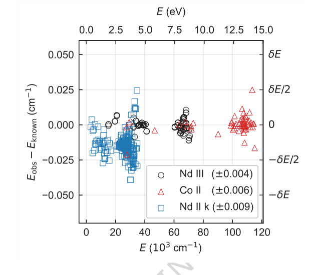Figure 4. Difference between energy levels determined from a single seed and their known (ac- cepted) values for each species. Only levels contributing to Nc are shown. Energy differences for Nd III, Co II, and Nd II k are shown in circles, triangles, and squares, respectively. The root-mean-square energy differences are given in parentheses in the legend. Typical energy level uncertainty by FT spectroscopy is of order 0.001 cm−1. The offset and higher spread of Nd II k energies are expected and within uncertainties as their known values were derived by lower-precision grating spectroscopy [4]

Mathematical & Logical Mechanism

The Master Equation

The core of this paper's mechanism revolves around two fundamental equations: the objective function for the Markov Decision Process (MDP) that the agent aims to maximize, and the loss function that drives the learning of the underlying neural network. Additionally, a crucial calculation for determining energy levels forms an integral part of the state update mechanism.

The primary objective of the reinforcement learning agent is to maximize the expected cumulative discounted reward over a finite horizon $H$:

$$ E[G_t] = E\left[\sum_{k=0}^{H} \gamma^k r_{t+k}\right] \quad (1) $$

This equation defines what the agent is trying to achieve: making a sequence of decisions that lead to the highest possible sum of future rewards, where rewards received sooner are valued more highly than those received later.

The learning process for the Deep Q-Network (DQN) agent is driven by minimizing a loss function, specifically the squared n-step Temporal Difference (TD) error:

$$ L = [TD[n]]^2 = \left[r^{[n]} + \gamma^n Q_{\bar{\theta}}(s_{t+n}, \text{argmax}_{a_{t+n}} Q_{\theta}(s_{t+n}, a_{t+n})) – Q_{\theta}(s_t, a_t)\right]^2 \quad (15) $$

This loss function guides the neural network to accurately predict the "quality" of actions, ensuring that its estimates align with actual future rewards.

Finally, a critical calculation that underpins the state updates, particularly the determination of observed energy levels ($E_{obs}$), is performed via weighted least-squares minimization:

$$ E_{obs} = \text{argmin}_{E_n} \sum_{m=0}^{M-1} w_m \left( \sum_{n=0}^{N-1} S_{mn}E_n - \sigma_m \right)^2 \quad (9) $$

This equation is how the system refines the energy values of known levels based on observed spectral lines, making it a central component of the "mathematical engine" that processes and updates the atomic data.

Term-by-Term Autopsy

Let's dissect each of these equations to understand their individual components and their roles.

Equation (1): Expected Cumulative Discounted Reward

• $E[G_t]$: This represents the expected cumulative discounted reward starting from time step $t$.
  • Mathematical Definition: The average value of $G_t$ over many possible trajectories.
  • Physical/Logical Role: This is the ultimate objective function for the reinforcement learning agent. The agent's policy is designed to choose actions that maximize this quantity, effectively finding the best sequence of decisions to determine atomic fine structures.
• $E[\cdot]$: This is the expectation operator.
  • Mathematical Definition: Calculates the average value of a random variable.
  • Physical/Logical Role: In reinforcement learning, the agent doesn't know the exact future rewards or state transitions deterministically. This operator accounts for the inherent uncertainty in the environment, ensuring the agent optimizes for the average outcome.
• $G_t$: This is the cumulative discounted reward from time $t$.
  • Mathematical Definition: The sum of all future rewards, each discounted by a factor $\gamma$ raised to the power of the number of steps into the future.
  • Physical/Logical Role: It quantifies the total "goodness" of a particular sequence of actions and states starting from time $t$.
• $\sum_{k=0}^{H} \gamma^k r_{t+k}$: This is the summation of discounted future rewards.
  • Mathematical Definition: A finite sum where each reward $r_{t+k}$ is multiplied by $\gamma^k$.
  • Physical/Logical Role: It aggregates the rewards obtained at future time steps $t+k$, applying a discount to make immediate rewards more valuable than distant ones. The summation is used because the total reward is an accumulation of individual rewards.
• $\gamma$: This is the discount factor.
  • Mathematical Definition: A scalar value between 0 and 1 (inclusive), $\gamma \in [0, 1]$.
  • Physical/Logical Role: It balances the importance of immediate rewards versus future rewards. A $\gamma$ closer to 0 makes the agent "myopic," focusing on immediate gains, while a $\gamma$ closer to 1 makes it "far-sighted," considering long-term consequences. The authors chose addition for the sum because the total value is an accumulation of individual rewards.
• $k$: This is the time step index relative to $t$.
  • Mathematical Definition: An integer representing the number of steps into the future from time $t$.
  • Physical/Logical Role: It tracks how far into the future a particular reward $r_{t+k}$ is received, which determines the power to which $\gamma$ is raised for discounting.
• $r_{t+k}$: This is the reward received at time $t+k$.
  • Mathematical Definition: A scalar value representing the immediate feedback from the environment after taking an action.
  • Physical/Logical Role: In this paper, rewards are designed to reflect confidence in determined energy levels, agreement with theory and observations, and the ability to enable future level determinations (equations 6 and 7).

Equation (15): Loss Function for TAG-DQN

• $L$: This is the loss function.
  • Mathematical Definition: A scalar value quantifying the error between the predicted Q-values and the target Q-values.
  • Physical/Logical Role: The goal of training is to minimize this loss, which in turn makes the Q-network's predictions more accurate.
• $[TD[n]]^2$: This is the squared n-step Temporal Difference (TD) error.
  • Mathematical Definition: The square of the difference between the n-step return (an estimate of future reward) and the current Q-value prediction.
  • Physical/Logical Role: Squaring the error ensures that both positive and negative errors contribute to the loss and penalizes larger errors more heavily, promoting convergence.
• $r^{[n]}$: This is the n-step return.
  • Mathematical Definition: The sum of the first $n$ rewards, discounted, plus the discounted Q-value of the state reached after $n$ steps.
  • Physical/Logical Role: It provides a more stable and less biased estimate of the true value compared to a single-step return, by incorporating actual rewards over a short horizon before bootstrapping from a Q-value estimate.
• $\gamma^n$: This is the discount factor raised to the power of $n$.
  • Mathematical Definition: The discount factor $\gamma$ multiplied by itself $n$ times.
  • Physical/Logical Role: It discounts the future Q-value estimate at state $s_{t+n}$ back to time $t$, aligning its value with the rewards received over the $n$ steps.
• $Q_{\bar{\theta}}(s_{t+n}, \text{argmax}_{a_{t+n}} Q_{\theta}(s_{t+n}, a_{t+n}))$: This is the target Q-value.
  • Mathematical Definition: The Q-value of state $s_{t+n}$ and the action that maximizes the Q-value in that state, as predicted by the target network $Q_{\bar{\theta}}$.
  • Physical/Logical Role: This term provides a stable target for the online network to learn from. By using a separate target network with delayed updates ($\bar{\theta}$), it prevents the Q-value estimates from chasing a moving target, which can lead to instability in training. The $\text{argmax}$ part ensures that the target reflects the value of the best possible action from the next state, according to the online network's current understanding.
• $Q_{\theta}(s_t, a_t)$: This is the current Q-value prediction.
  • Mathematical Definition: The Q-value of the current state-action pair $(s_t, a_t)$, as predicted by the online network $Q_{\theta}$.
  • Physical/Logical Role: This is the value the network is currently predicting for taking action $a_t$ in state $s_t$. The loss function aims to adjust $\theta$ so this prediction matches the target Q-value.
• $s_t$: This is the state at time $t$.
  • Mathematical Definition: A representation of the environment at time $t$, including graph nodes and edge features (equations 2 and 3).
  • Physical/Logical Role: It encapsulates all relevant information about the current term analysis progress, such as known/unknown levels, observed spectral lines, and theoretical calculations.
• $a_t$: This is the action taken at time $t$.
  • Mathematical Definition: A discrete choice made by the agent, either selecting an unknown level ($a^{(1)}$) or matching lines to determine its energy ($a^{(2)}$).
  • Physical/Logical Role: It represents the agent's decision in the term analysis process.
• $\theta$: These are the parameters of the online Q-network.
  • Mathematical Definition: The weights and biases of the neural network that currently predicts Q-values.
  • Physical/Logical Role: These are the parameters that are actively updated during training to improve the agent's policy.
• $\bar{\theta}$: These are the parameters of the target Q-network.
  • Mathematical Definition: The weights and biases of a copy of the Q-network, updated less frequently or smoothly.
  • Physical/Logical Role: Provides a stable reference for the target Q-values, crucial for the stability of the learning process.
• $\text{argmax}_{a_{t+n}} Q_{\theta}(s_{t+n}, a_{t+n})$: This operator finds the action that maximizes the Q-value in state $s_{t+n}$ according to the online network.
  • Mathematical Definition: Returns the action $a_{t+n}$ that yields the highest Q-value for state $s_{t+n}$ using the online network parameters $\theta$.
  • Physical/Logical Role: This is a key component of Double DQN, where the online network selects the action for the target value calculation, but the target network evaluates its value. This helps to mitigate overestimation bias in Q-learning.

Equation (9): Level Energy Optimization

• $E_{obs}$: This represents the observed energies of the levels.
  • Mathematical Definition: A vector of energy values $E_n$ for $N$ known levels.
  • Physical/Logical Role: These are the empirically determined energy levels that the term analysis aims to establish.
• $\text{argmin}_{E_n}$: This is the minimization operator.
  • Mathematical Definition: Finds the values of $E_n$ that minimize the subsequent expression.
  • Physical/Logical Role: It signifies that the observed energy levels are determined by finding the set of energies that best fit the observed spectral lines, minimizing the discrepancies.
• $\sum_{m=0}^{M-1} w_m \left( \sum_{n=0}^{N-1} S_{mn}E_n - \sigma_m \right)^2$: This is the weighted sum of squared residuals.
  • Mathematical Definition: A sum over all $M$ known lines, where each term is the squared difference between a predicted wavenumber and an observed wavenumber, weighted by $w_m$.
  • Physical/Logical Role: This is the objective function for the least-squares optimization. It quantifies the overall disagreement between the current set of energy levels and the observed spectral lines. Minimizing this sum means finding the energy levels that best explain the observed spectrum. The summation is used because the total error is an aggregate of errors from individual lines.
• $M$: This is the total number of known lines.
  • Mathematical Definition: An integer count of the spectral lines that have been matched to transitions between known energy levels.
  • Physical/Logical Role: Represents the amount of empirical data available to constrain the energy levels.
• $N$: This is the total number of known levels.
  • Mathematical Definition: An integer count of the energy levels whose values are being optimized.
  • Physical/Logical Role: Represents the number of atomic energy states whose values are being refined.
• $w_m$: This is the weight for line $m$.
  • Mathematical Definition: $w_m = (\delta\sigma_m)^{-2}$, the inverse square of the wavenumber uncertainty for line $m$.
  • Physical/Logical Role: It assigns higher importance to more precisely measured spectral lines (those with smaller $\delta\sigma_m$) and less importance to lines with higher uncertainty. This ensures that reliable data has a greater influence on the determined energy levels. The inverse square is a standard choice in weighted least squares, where weights are inversely proportional to the variance of the measurement error.
• $\left( \sum_{n=0}^{N-1} S_{mn}E_n - \sigma_m \right)^2$: This is the squared difference (residual) for line $m$.
  • Mathematical Definition: The square of the difference between the wavenumber predicted by the current energy levels and the observed wavenumber for line $m$.
  • Physical/Logical Role: It measures how well the current set of energy levels explains a specific observed spectral line. Squaring ensures positive values and penalizes larger deviations more.
• $S_{mn}$: This is the coefficient defining the relationship between energy levels and line $m$.
  • Mathematical Definition: A matrix element that is 1 if level $n$ is the upper level of transition $m$, -1 if level $n$ is the lower level of transition $m$, and 0 otherwise.
  • Physical/Logical Role: This coefficient encodes the fundamental relationship that a spectral line's wavenumber ($\sigma_m$) is the difference between the upper ($E_u$) and lower ($E_l$) energy levels involved in the transition: $\sigma_m = E_u - E_l$.
• $E_n$: This is the energy of level $n$.
  • Mathematical Definition: A scalar value representing the energy of a specific atomic level.
  • Physical/Logical Role: These are the unknown parameters that the optimization process aims to determine.
• $\sigma_m$: This is the observed wavenumber for line $m$.
  • Mathematical Definition: A measured scalar value representing the wavenumber of a spectral line.
  • Physical/Logical Role: This is the empirical input data from the spectral line list that the energy levels must conform to.

Step-by-Step Flow

Imagine the term analysis as a dynamic assembly line, where an abstract data point, representing the current state of atomic level determination, moves through a series of operations.

1. Initial State Input: The process begins with an initial graph state $s_t$. This state is a rich data structure, a graph $G=(V, E)$, where nodes $V$ are atomic energy levels (some known, some unknown) and edges $E$ are potential or observed spectral lines (transitions). Each node and edge carries a set of features (e.g., theoretical energies, observed wavenumbers, uncertainties, binary flags for "known" or "selected"). Alongside this, there's a comprehensive spectral line list containing all observed transitions.

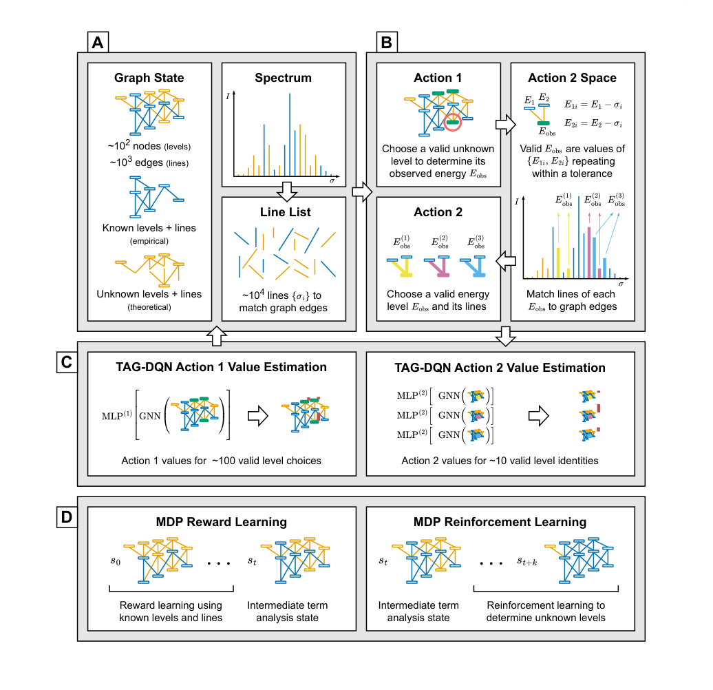Figure 1. Illustration of the MDP environment and TAG-DQN. A The term analysis state is represented as a graph with node and edge features, alongside the spectral line list. B Actions alternate between two regimes; each pair of actions leads to the determination of the observed energy Eobs for one level by matching at least two lines from the line list to unknown edges in the graph. C TAG-DQN employs a GNN to embed graph representations, which are inputs for multilayer perceptrons (MLPs) estimating Q-values for each action (vertical bars); the highest Q-value action advances the MDP to the next state. D Given a term analysis state st, the MDP trajectory leading to st involving known levels is used for reward learning, while RL with the learned reward function guides the discovery of unknown levels in future states st+k

1. Action $a^{(1)}$: Level Selection: The agent first performs an action of type $a^{(1)}$. It surveys all currently unknown levels that have at least two potential connections (edges) to known levels. From this pool, the agent selects one specific unknown level to focus on for determination. This selection is based on the agent's learned Q-values, which estimate the long-term reward of choosing that level. Once selected, a "selected" flag for this node is flipped to indicate it's the current target.

2. Action $a^{(2)}$: Line Matching & Energy Hypothesis: Next, the agent executes an action of type $a^{(2)}$. For the "selected" unknown level, it considers all possible edges connecting it to known levels. For each such edge, it filters the entire spectral line list (which can contain $10^4$ lines) to find candidate observed lines. This filtering is strict:

   • Wavenumber Match: An observed wavenumber $\sigma_{obs}$ must fall within a theoretical range $[\sigma_{calc} \pm \Delta E]$, where $\sigma_{calc}$ is the theoretical wavenumber for the transition and $\Delta E$ is the energy uncertainty.
   • Intensity Match: The observed intensity $I_{obs}$ must be within a theoretical range $[I_{calc} \pm \Delta I]$.
   • Candidate $E_{obs}$ Generation: For each filtered line, a candidate observed energy $E_{obs}$ for the selected unknown level is calculated by adding or subtracting the line's wavenumber from the known energy of the connected level (depending on whether the selected level is upper or lower).
   • Consolidation: Since multiple lines might suggest the same energy for the unknown level, candidates are grouped, and only $E_{obs}$ values that repeat within a small tolerance $\delta E$ are considered. The agent then chooses one of these consolidated $E_{obs}$ values (or a "no-op" if no suitable candidates exist).

3. State Transition & Graph Update: Once an $E_{obs}$ value is chosen for the selected level (via $a^{(2)}$), the graph state $s_t$ deterministically transitions to a new state $s_{t+1}$:

   • The "selected" unknown level now becomes a "known" level, and its $E_{obs}$ feature is updated with the chosen value.
   • The edges corresponding to the matched spectral lines also become "known" edges, and their features (e.g., $\sigma_{obs}$, $I_{obs}$) are updated from the line list. These matched lines are then excluded from future $a^{(2)}$ considerations in this episode.
   • Global Re-optimization: Crucially, after a new level is determined, the observed energies $E_{obs}$ for all currently known levels (including the newly determined one) are re-optimized using the weighted least-squares minimization (Equation 9). This ensures consistency across the entire known level system. The ground energy level $E_0$ is fixed at zero as a reference.

4. Reward Calculation: Based on the new state $s_{t+1}$ and the actions taken, a reward $r_t$ is calculated. This reward is a composite, reflecting the confidence in the determined level, its agreement with theory, and its potential to enable future determinations. For $a^{(1)}$, it's based on the signal-to-noise ratio of connecting lines (Equation 6). For $a^{(2)}$, it incorporates a learned preference score $D$ (Equation 7), which is derived from human expert decisions.

5. Experience Storage: The tuple $(s_t, a_t, r_t, s_{t+1})$ – representing the old state, action taken, reward received, and new state – is stored in a replay buffer. This buffer acts as a memory, accumulating past experiences.

6. Iteration: The process then loops back to step 2, with the agent selecting another unknown level or continuing to refine the current one, until a finite horizon $H$ is reached or no more valid actions can be taken.

This entire sequence makes the abstract math feel like a moving mechanical assembly line, where raw spectral data is continuously refined and integrated into a growing, self-consistent model of atomic energy levels.

Optimization Dynamics

The TAG-DQN mechanism learns and converges through a sophisticated interplay of deep reinforcement learning techniques, primarily driven by minimizing the Temporal Difference (TD) error. Here's how it works:

1. Graph Representation Learning: The foundation is a Graph Neural Network (GNN). When a graph state $s_t$ (representing the current set of known/unknown levels and lines) is presented, the GNN processes its nodes (levels) and edges (lines) and their associated features (e.g., $E_{calc}$, $\sigma_{obs}$, $I_{obs}$). It uses multi-head graph attention layers to learn rich, contextual node embedding vectors $h_v$ for each level $v$. These embeddings capture the structural and feature information of the local neighborhood around each node. A global graph state embedding vector $S_{agg}$ is then obtained by simply averaging these node embeddings (Equation 11). This $S_{agg}$ effectively summarizes the entire graph's current state.

2. Q-Value Estimation (Duelling DQN): The learned graph embeddings are then fed into Multi-Layer Perceptrons (MLPs) to estimate Q-values. The architecture employs a Duelling DQN design, which separates the estimation of the state-value function $V(s)$ and the advantage function $A(s, a)$.

   • For action type $a^{(1)}$ (selecting an unknown level), the Q-value for each valid level choice is estimated by combining the global $S_{agg}$ (for the state-value) with the node embedding of the chosen level (for the advantage), as shown in Equation (12).
   • For action type $a^{(2)}$ (matching lines to determine an energy), the Q-value is estimated similarly, but the advantage function $A(s,a)$ is computed by taking the difference between the state-action value and the state value, as shown in Equation (13). This separation helps the network learn which states are valuable independently of the actions taken, improving efficiency.

3. Policy and Exploration: The agent's policy is greedy with respect to the estimated Q-values. At each step, it selects the action (either $a^{(1)}$ or $a^{(2)}$) that has the highest predicted Q-value. For exploration, instead of the traditional epsilon-greedy method, the authors use noisy networks. This means that noise is added directly to the weights of the MLP output layers, encouraging the agent to explore different actions naturally without needing an explicit $\epsilon$ parameter. The noise is learned and adapted over time, allowing for more efficient exploration in complex environments.

4. Learning from Experience (Replay Buffer & n-step Returns): To learn, the agent doesn't just use its most recent experience. Instead, it stores past experiences (state, action, reward, next state tuples) in a replay buffer. During training, batches of these experiences are randomly sampled from the buffer. This breaks correlations between consecutive experiences, stabilizing the learning process. The loss calculation (Equation 15) uses n-step returns ($r^{[n]}$), which means that instead of just considering the immediate reward $r_t$ and the Q-value of the next state $s_{t+1}$, it looks $n$ steps into the future. This provides a more accurate target for learning by incorporating actual rewards over a short trajectory before bootstrapping from a Q-value estimate.

5. Target Network for Stability: A key challenge in Q-learning is that the target value (what the network is trying to predict) depends on the same network that is being updated, leading to instability. To address this, TAG-DQN uses a target network $Q_{\bar{\theta}}$. This is a separate copy of the online Q-network ($Q_{\theta}$) whose parameters $\bar{\theta}$ are updated much more slowly than $\theta$. Specifically, $\bar{\theta}$ is soft-updated (Equation 14) by blending a small fraction of the online network's parameters into the target network's parameters at each step. This creates a stable target for the online network to learn from, preventing oscillations and divergence. The use of Double DQN further refines this by using the online network to select the best action for the next state, but the target network to evaluate its value, which helps to mitigate overestimation bias.

6. Reward Function Learning (Inverse Reinforcement Learning): A unique aspect is that the reward function for action $a^{(2)}$ (the preference score $D$) is not hand-coded. Instead, it's learned from historical human expert decisions using a form of inverse reinforcement learning. A simple multi-layer perceptron (MLP) is trained to predict $D$ from features of the candidate lines (Equation 8). This MLP is trained on expert-generated MDP state transitions, where human choices are labeled as positive examples. This allows the system to implicitly capture the nuanced judgment of human experts regarding the "goodness" of a particular line match, shaping the loss landscape to favor actions that align with expert intuition.

7. Optimization Algorithm: The network parameters $\theta$ are optimized using the Adam optimizer, a popular stochastic gradient descent method known for its efficiency and good performance in deep learning tasks. This iterative optimization process adjusts the weights and biases of the GNN and MLPs to minimize the loss function, thereby improving the accuracy of Q-value predictions and, consequently, the agent's policy.

In essence, the optimization dynamics involve a continuous cycle: the agent acts in the environment, collects experience, stores it, and then learns from batches of this experience by minimizing a carefully constructed loss function. This learning process is stabilized by techniques like target networks, n-step returns, and duelling architectures, while exploration is handled by noisy networks. The learned reward function, derived from human expertise, further guides the agent towards physically meaningful solutions, shaping the loss landscape to reflect expert preferences and uncertainties. This iterative refinement allows the agent to converge towards a policy that efficiently and accurately determines atomic fine structures.

Results, Limitations & Conclusion

Experimental Design & Baselines

To rigorously validate their mathematical claims, the authors architected a series of experiments comparing their Term Analysis with Graph Deep Q-Network (TAG-DQN) against two baseline models: a greedy search agent and a standard Monte-Carlo Tree Search (MCTS) agent, which employed the Upper Confidence Bound for Trees (UCT) strategy. The core idea was to demonstrate that TAG-DQN could effectively automate and accelerate the complex, sequential decision-making task of atomic fine structure determination.

The experimental setup involved four distinct Markov Decision Process (MDP) environments, each derived from real-world atomic term analyses of Co II, Nd III, and two variants of Nd II (Nd II u for ab initio calculations and Nd II k for Cowan code calculations). These environments were carefully constructed to reflect the challenges of actual term analysis, using existing Fourier Transform (FT) spectral line lists and theoretical calculations. For instance, the Co II environment was initialized with 141 known levels from revised published data, while Nd III used 40 levels. The Nd II environments started with six ground term levels, five 6K levels, and 11 transitions, differing in their theoretical calculation methods.

To ensure a fair and robust comparison, TAG-DQN and MCTS were evaluated across 25 different random seeds, with average performance and 95% confidence intervals reported. The greedy search, being deterministic, was run once. Performance was measured using three key metrics:
1. $R_{max}$: The maximum cumulative reward achieved by an agent within an MDP episode of length $H$.
2. $N_c$: The number of correctly determined energy levels in the $R_{max}$ episode, where a level was considered correct if its observed energy ($E_{obs}$) was within $\pm \delta E$ of a previously published energy level ($E_{known}$).
3. Accuracy (Acc.): Defined as the ratio of $N_c$ to the total number of levels determined in the $R_{max}$ episode.

The MDP environments were carefully simplified to enhance feasibility and RL performance. This involved pruning graph edges with low signal-to-noise ratios ($S/N_{calc} < 2$), excluding line list entries already matched, fixing initial known levels during energy optimization, and limiting spectral ranges. A maximum cap on the action space for matching lines ($|A^{(2)}|$) was also imposed to aid efficient exploration and manage memory. The episode length $H$ was varied per species (e.g., $H=128$ for Nd III and Co II, $H=64$ for Nd II u, $H=512$ for Nd II k) to balance computational cost with the agent's ability to learn long-term consequences.

Furthermore, ablation studies were conducted on the Nd III environment to dissect the contribution of various Deep Q-Network (DQN) extensions (such as double Q-learning, prioritized experience replay, dueling, multi-step returns, and noisy networks for exploration) to TAG-DQN's overall performance. This allowed the researchers to pinpoint which architectural components were most crucial for the model's succesful operation.

What the Evidence Proves

The experimental results provide compelling evidence that TAG-DQN can significantly accelerate atomic fine structure determination, a task traditionally requiring months to years of human effort. The system was able to identify and determine hundreds of energy levels in a matter of hours.

Specifically, the core mechanism of TAG-DQN, which casts term analysis as a Markov decision process solved by graph reinforcement learning with a reward function partly learned from human decisions, demonstrably worked in reality. The definitive evidence lies in the high agreement rates with published values: 95% for Co II and between 54% and 87% for Nd II and Nd III. This level of accuracy, achieved in a fraction of the time, is a strong indicator of the method's efficacy.

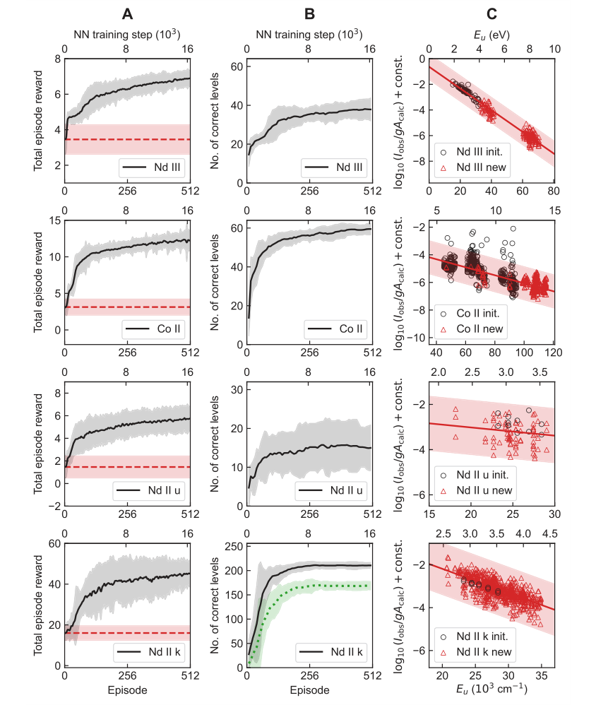Figure 2. Learning results of TAG-DQN agent in the four case studies of Table 1. A Average learning curves, i.e., mean cumulative rewards obtained as a function of neural network (NN) training steps. The dashed horizontal lines show reward obtained during the pre-training episodes and correspond to rewards obtained by choosing actions in the MDP uniformly at random. The shaded regions show ±2 standard deviations across 25 random seeds. B Average Nc of the final state of the most recent maximum reward episode. The dotted curve for Nd II k shows the number of correct levels that also match human chosen level labels, and the y-axes limits are H

When pitted against the baseline models (Table 2), TAG-DQN consistently outperformed the greedy search agent across all metrics. More importantly, it showed superior performance over the MCTS agent in terms of $N_c$ (number of correctly determined levels) in three out of five case studies. While MCTS sometimes achieved a higher maximum cumulative reward ($R_{max}$), TAG-DQN consistently reached higher upper bounds for $N_c$, particularly in the Nd II cases. This suggests that TAG-DQN was better at choosing level identities that remained consistent with observations and theory throughout an episode, whereas MCTS's shallower rollouts might have favored short-term rewards at the expense of overall accuracy. For Nd II k, TAG-DQN correctly labeled a significantly larger number of levels (169 $\pm$ 10) compared to MCTS (130 $\pm$ 11), further reinforcing this interpretation.

The learning curves (Figure 2A, B) clearly illustrate the alignment between the cumulative reward and the number of correctly determined levels ($N_c$), indicating that the learned reward function effectively guides the agent towards accurate level determinations. The Boltzmann plots (Figure 2C) confirmed that TAG-DQN could determine levels across different electron configurations and that its line intensity filtering, based on Boltzmann level populations, was effective in excluding problematic lines.

The ablation studies (Figure 3) provided crucial insights into TAG-DQN's architecture. They revealed that most DQN extensions contributed positively to performance, with dueling network architectures and noisy networks for exploration being particularly critical. This is likely due to the large action spaces inherent in the problem. Interestingly, prioritized experience replay (PER) slightly reduced performance, possibly because the buffer size and training steps were not optimally scaled for PER's benefits in this specific environment. The energy level differences (Figure 4) further supported the method's precision, showing that while a small fraction of determined levels deviated from accepted values, these deviations were generally within the experimental uncertainty $\delta E$ (e.g., $\pm 0.004$ cm$^{-1}$ for Nd III, $\pm 0.006$ cm$^{-1}$ for Co II, $\pm 0.009$ cm$^{-1}$ for Nd II k), making them negligible for most applications.

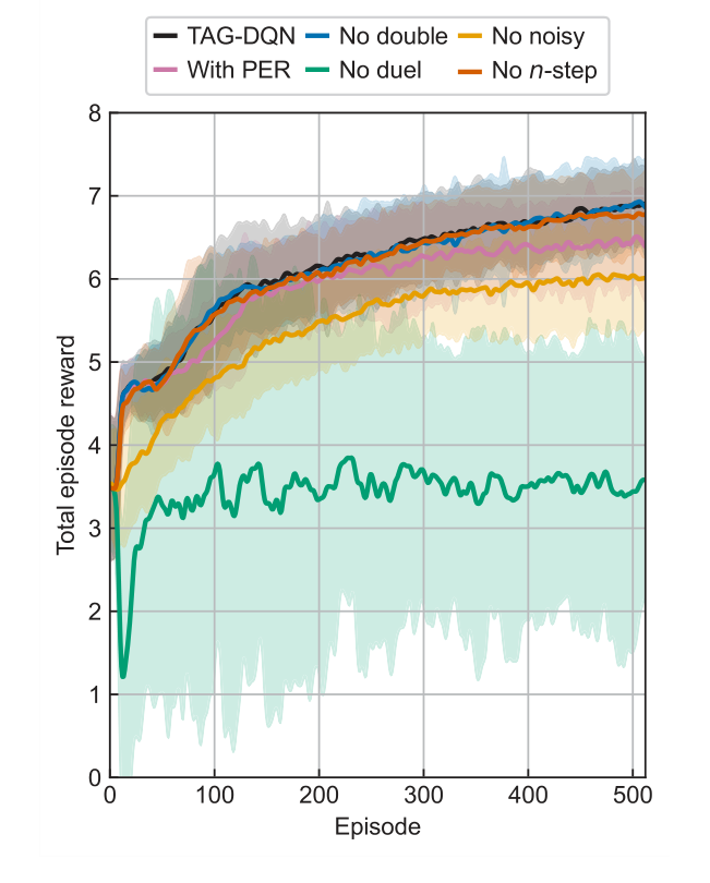Figure 3. Learning curves of TAG-DQN (black) and its variants in the Nd III environment. Average total episode reward during training of TAG-DQN and its designs with or without particular deep Q-network extensions: without double Q-learning (blue), without noisy networks for exploration (yellow), with prioritised experience replay (PER, pink), without duelling deep Q-network (green), and without multi(n)-step return (orange). Shaded regions show ±2 standard deviations across 16 seeds. The duelling extension and noisy networks for exploration are key for TAG-DQN, while using PER reduced performance slightly

Limitations & Future Directions

While the TAG-DQN approach marks a significant stride in automating atomic fine structure determination, it's important to acknowledge its current limitations and consider avenues for future development.

One primary limitation is that the current method, despite its impressive speed, still exhibits reduced accuracy compared to human experts and relies on atomic structure calculations. The determined levels, especially for cases like Nd II k, are considered tentative and require human validation before final publication. Furthermore, the current framework does not yet tackle the most challenging scenarios in term analysis, such as determing single-line levels, connecting disconnected known-level subgraphs, or initiating analyses from a completely unknown state. These situations would significantly increase MDP complexity and necessitate substantial redesign. The reward function, currently trained predominantly on Co II data, could benefit from a more diverse and extensive training dataset to improve its generalization across different atomic species and conditions.

Looking ahead, several promising directions could further evolve these findings:

• Enriching the MDP State and Action Space: The current MDP could be expanded to incorporate more granular information. For instance, integrating raw spectrum and line profile analysis directly into the MDP would allow the agent to consider additional factors like isotope shifts, hyperfine structure, and comparisons across different spectra. Information about the wavefunction, such as leading configuration labels, electron probability density, and local level density within specific parity and J values, could also inform the agent's decisions on line profiles and intensities, potentially leading to more robust and accurate level determinations.
• Developing a More Robust Reward Function: As noted, the current reward function's reliance on a limited dataset is a constraint. Future work should focus on training a more generalized reward function using a vast array of line lists and MDPs from diverse atomic species. This would enhance the agent's ability to handle novel situations and improve overall performance.
• Human-in-the-Loop Integration: The authors envision a collaborative approach where the AI's output serves as an intermediate step. The final MDP state of an episode could become a new initial state for human experts to inspect the spectrum, prune incorrectly determined levels, refine semi-empirical calculations, and retrain the reward function. This iterative human-AI collaboration could leverage the strengths of both, with the AI handling the laborious initial identification and the human expert providing critical validation and refinement.
• Addressing Complex Scenarios: Future research should focus on redesigning the MDP to handle the currently omitted challenging situations. This might involve novel graph representations or action space decompositions to manage the increased complexity, potentially unlocking the ability to automate even the most difficult aspects of term analysis.
• Extending to Other Experimental Methods: The approach is inherently flexible and could be adapted to other experimental methods, such as grating spectroscopy, with minor adjustments to environment parameters like $\delta E$, $\Delta I$, and the reward function. This would broaden the applicability of graph reinforcement learning across various spectroscopic techniques.
• Computational Efficiency and Infrastructure: While TAG-DQN can run on commodity hardware for single-seed runs, comprehensive experiments involving extensive hyperparameter tuning and multi-seed evaluations demand significant computational resources. Future work could explore more efficient hyperparameter optimization techniques or distributed computing frameworks to reduce the computational cost and time required for extensive research.

Ultimately, this work is a testament to the potential of graph reinforcement learning and AI in general to assist scientific discovery, particularly in data- and labor-intensive fields. The proposed advancements could pave the way for a new era of accelerated atomic physics research, closing the gap between the demand for atomic data and the current efficiency of its determination.

Table 2. Results and comparisons with benchmark agents. TAG-DQN matches MCTS performance as judged by downstream metrics in 2/5 cases and outperforms it in 3/5 cases, while Greedy search is worse overall 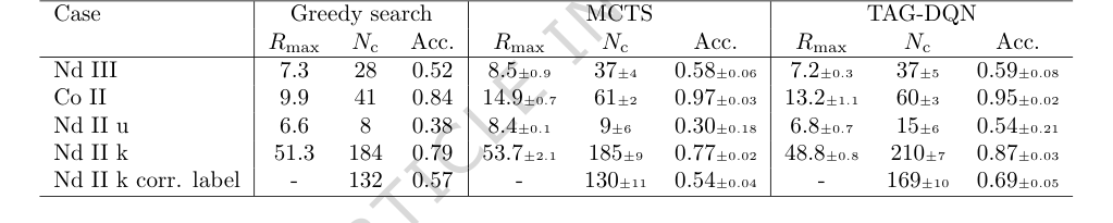Table 1. Key term analysis MDP environment parameters