Localising entropy production along non-equilibrium trajectories

Background & Academic Lineage

The Origin & Academic Lineage

The problem at the heart of this paper originates from a fundamental and long-standing challange in non-equilibrium statistical physics: how to precisely quantify and spatiotemporal localizaton the irreversibility and energy dissipation within complex systems, directly from experimentally observed data. While the concept of entropy production serves as a universal metric for these phenomena, its precise localization in space and time along non-equilibrium trajectories has remained a significant "open challenge" (Page 2).

Historically, the academic lineage traces back to the advancements in stochastic thermodynamics [17-19] and the emergence of data-driven approaches [11, 20-23]. These fields provided a rigorous framework for understanding entropy production in individual realizations of non-equilibrium processes, especially when thermal fluctuations are prominent [18, 26]. However, a major hurdle persisted: conventional methods for measuring entropy production or dissipative force fields typically relied on pior knowledge of the system's underlying dynamical equations, such as Fokker-Planck or Master equations. In many realistic experimental scenarios, these equations and their solutions are unknown, rendering traditional approaches impractical (Page 2).

Previous research predominantly focused on obtaining global estimates of the average entropy production rate. While methods like the Harada-Sasa equality [6], steady-state current estimations [5], time-irreversibility measures [26-31], and path probability estimators [4, 32, 33] offered valuable insights, they generally provided an overall measure rather than a detailed, localized picture of dissipation. Attempts to localize entropy production were often limited: for example, brute-force statistical binning [20] scaled poorly with higher-dimensional systems, and some neural network approaches learned entropy production along trajectories but did not fully elucidate the structure of the underlying dissipative force fields [23]. Other methods could only infer parts of the dissipative force field, assuming the remaining components were already known [11, 40]. The fundamental limitation, or "pain point," that this paper seeks to address is the lack of a robust, scalable, and model-free method to infer the spatiotemporal structure of both the dissipative force field and the fluctuating entropy production directly from experimental trajectory data, particularly in complex, high-dimensional, and time-dependent non-equilibrium systems, without requiring explicit knowledge of their governing dynamics. This critical gap motivated the development of the data-driven approach presented here, which leverages the thermodynamic uncertainty relation (TUR) and machine learning.

Intuitive Domain Terms

• Entropy Production ($\sigma$): Imagine a perfectly organized room. If you throw a party, things get messy. The "entropy production" is like the amount of irreversible mess created during the party. A higher value means more chaos and a greater inability to easily return the room to its original state.
• Non-equilibrium Trajectories: Think of a person walking through a crowded market. They are constantly moving, bumping into people, changing direction, and never truly standing still in a balanced state. A "non-equilibrium trajectory" is the specific, winding path that person takes, always in motion and interacting with their surroundings.
• Thermodynamic Force Field ($F(\mathbf{x}, t)$): This is like the invisible "current" or "wind" that pushes and pulls objects in a complex environment, making them move in a particular, often swirling, way. It's not just a simple push, but a dynamic, spatially varying influence that drives the system away from a calm, balanced state and causes energy to be dissipated.
• Thermodynamic Uncertainty Relation (TUR): Consider a tightrope walker. The "TUR" is like a fundamental rule that says, "The faster you try to cross the rope (higher entropy production), the more your body will sway and wobble (larger fluctuations in your movement are inevitable)." It establishes a trade-off between how efficiently you perform an irreversible task and how predictably your path will be.
• Overdamped Diffusive Processes: Picture a tiny feather slowly drifting down through still air. Its fall is entirely dictated by air resistance and random air currents, not by its own momentum. An "overdamped diffusive process" describes movement where inertia is negligible, and motion is dominated by friction and random pushes from the environment.

Notation Table

Notation	Description

Problem Definition & Constraints

Core Problem Formulation & The Dilemma

The core problem this paper tackles is the precise, spatiotemporal localization of entropy production and the underlying dissipative force fields in complex non-equilibrium systems, derived directly from experimentally measured trajectory data.

Input/Current State: The starting point for this analysis is raw, experimentally measurable trajectory data, $\mathbf{x}(t)$, of a system operating far from thermodynamic equilibrium. A crucial aspect is that this data is assumed to be available without prior knowledge of the system's underlying dynamical equations (such as Fokker-Planck or Master equations) or their analytical solutions, nor the specific system parameters.

Output/Goal State: The desired endpoint is a detailed, localized understanding of the system's irreversibility. This includes:
1. The dissipative (thermodynamic) force field, $F(\mathbf{x},t)$, which is the driving force behind the non-equilibrium dynamics.
2. The corresponding fluctuating entropy production, $\sigma$, localized in both space and time along individual trajectories. This output allows researchers to pinpoint when and where energy dissipation occurs within the system.

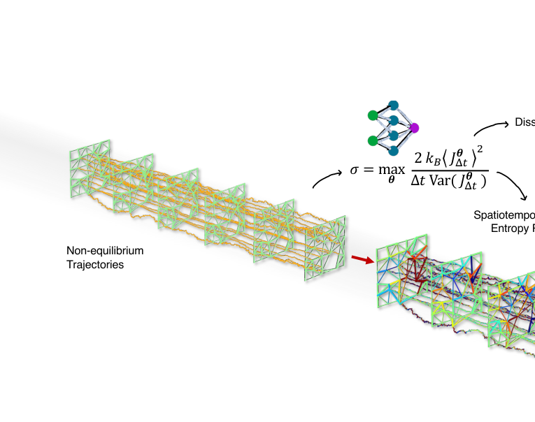FIG. 1. Schematic of entropy production inference in an active biological network model. Input: The method processes experimentally measurable trajectory data without requiring prior knowledge of system parameters. Outputs: Using short-time Thermodynamic Uncertainty Relations and neural networks (schematically illustrated at the top with a cartoon), we simultaneously infer (i) the dissipative (thermodynamic) force field F (x, t) driving the nonequilibrium dynamics and (ii) the corresponding fluctuating entropy production (color scale: ±0.015kB/s), localized in both space and time. Here, σ denotes the local entropy production rate, and J∆t represents a generalized current in phase space

Missing Link & Mathematical Gap: The fundamental gap lies in effectively translating raw trajectory data into these localized thermodynamic quantities. Historically, methods for quantifying entropy production have often relied on explicit knowledge of the system's dynamical equations, which are typically unknown or analytically intractable for complex, high-dimensional, or time-dependent systems. While global estimates of average entropy production rates can be obtained, extracting the spatiotemporal structure of fluctuating entropy production and the dissipative force field from data alone has remained a significant challenge.

This paper builds upon the short-time Thermodynamic Uncertainty Relation (TUR) as a variational principle. The TUR provides a formula for the entropy production rate, $\sigma_{TUR}(t)$, which can be maximized to yield the exact entropy production rate $\sigma(t)$. Crucially, the optimal coefficient field $d^*(\mathbf{x},t)$ that maximizes this relation is known to be proportional to the thermodynamic force field $F(\mathbf{x},t)$. The mathematical gap, then, is how to effectively learn this complex, potentially non-linear, and high-dimensional optimal coefficient field $d(\mathbf{x},t)$ directly from the trajectory data. The paper bridges this by employing deep neural networks to parameterize and infer $d(\mathbf{x},t)$, thereby reconstructing both the dissipative force field and the local entropy production.

The Dilemma: The central dilemma that has historically trapped researchers is the painful trade-off between the desire for high-resolution, localized information about entropy production and the practical limitations of analytical tractability and computational scalability. Previous approaches either:
* Required explicit knowledge of the system's dynamics, which is rarely available for realistic complex systems.
* Could only provide global, averaged entropy production rates, thus losing all spatiotemporal detail.
* Methods attempting to localize quantities, such as brute-force statistical binning, "scales poorly to higher dimensional systems" (Page 3), rendering them impractical for many real-world scenarios.
* Other data-driven methods might infer entropy production along trajectories but often "do not study the structure of the underlying dissipative force fields" (Page 3), which are essential for a complete understanding of the driving mechanisms. This paper aims to overcome this by offering a data-driven, model-free approach that provides both localized entropy production and the force field.

Constraints & Failure Modes

The problem of localizing entropy production from experimental trajectories is constrained by several harsh, realistic factors that make it insanely difficult to solve:

• Computational Complexity and High Dimensionality: Real-world non-equilibrium systems, particularly in fields like biology or active matter, often involve numerous interacting components, leading to high-dimensional phase spaces. The paper explicitly notes that "the complexity of high-dimensional, many-body interactions poses significant challenges for traditional optimization methods" (Page 5). Inferring complex, non-linear force fields in such vast spaces is computationally intensive and can quickly become intractable for methods that do not scale efficiently.
• Lack of A Priori Dynamical Knowledge: A major hurdle is the absence of known underlying dynamical equations (e.g., Fokker-Planck or Master equations) or their analytical solutions for most realistic systems (Page 2). This necessitates a model-free inference approach, which is inherently more challenging than parameter estimation within a pre-defined model.
• Time-Dependent Dynamics: Many non-equilibrium processes are explicitly time-dependent, meaning the thermodynamic force field and entropy production rate are also time-varying quantities. This temporal dependency "introduce significant computational challenges, making direct estimation of these quantities highly nontrivial" (Page 14). Training models to accurately capture such dynamic changes requires robust architectures and sufficient data.
• Data Quality and Signal-to-Noise Ratio (SNR): Experimental data is inherently noisy. A critical constraint arises in "weakly dissipative regions," where "irreversible signatures are small compared to fluctuations" (Page 10). In these low-dissipation regimes, the effective SNR for training the inference model is "strongly reduced," which "limit its ability to generalize uniformly across degrees of freedom with widely separated entropy production scales." This can lead to a mismatch between inferred and theoretical predictions in such regions, as illustrated in Figure 4(e).
• Experimental Sampling Limitations: The sampling interval, $\Delta t$, of experimental trajectories is "often fixed by practical constraints" (Page 5). While the short-time TUR ideally requires $\Delta t \to 0$ for exact saturation, practical $\Delta t$ values are finite. The method must be robust enough to handle these non-ideal sampling rates.
• Coarse-Graining and Hidden Degrees of Freedom: Experimental observations frequently provide only a "reduced description of the underlying dynamics" (Page 16). This can be due to "hidden degrees of freedom" (unobserved variables) or "finite temporal resolution" (subsampling). The inference method must be able to provide meaningful results even when the observed data is coarse-grained, which adds another layer of complexity to the problem.

Why This Approach

The Inevitability of the Choice

The authors' choice of combining the short-time Thermodynamic Uncertainty Relation (TUR) based inference scheme with deep neural networks was not merely an arbitrary selection but a necessary evolution driven by the inherent limitations of conventional approaches. The exact moment the authors realized traditional "SOTA" methods were insufficient for this specific problem is clearly articulated when they discuss the challenges of directly measuring entropy production and dissipative force fields from experimental data.

Traditional approaches, as the paper notes, "rely on the knowledge of the underlying dynamical equations, such as Fokker-Planck and Master equations, and their solutions, which are often unknown in realistic settings" (Page 2). This fundamental dependency on a priori knowledge of system dynamics renders them impractical for many real-world, complex systems where such equations are either too intricate to derive or simply unavailable. Furthermore, while some methods could provide global estimates of average entropy production, the critical need to "quantify and spatiotemporally localising it in complex processes directly from experimental data" (Page 2) remained a major open challenge. Previous attempts at localization, such as the brute-force statistical binning approach [20], "scales poorly to higher dimensional systems" (Page 3), indicating a lack of scalability. Other methods, like [23], learned entropy production along trajectories but failed to reveal the underlying dissipative force fields, which are crucial for understanding the dynamics.

The authors recognized that the problem's complexity, particularly in "high-dimensional, many-body interactions," posed "significant challenges for traditional optimization methods" (Page 5). This is the pivotal realization: existing methods, whether analytical or simpler statistical techniques, could not simultaneously infer both the local entropy production and the dissipative force field in a data-driven, scalable, and high-dimensional manner without prior knowledge of the system's governing equations. The short-time TUR, which provides a variational representation of the entropy production rate and links it directly to the thermodynamic force field (Eq. 9), offered the theoretical foundation. However, to practically solve this variational problem for complex, high-dimensional systems, a powerful function approximator was indispensable, leading directly to the adoption of deep neural networks.

Comparative Superiority

This combined approach demonstrates overwhelming qualitative superiority over previous gold standards, extending far beyond simple performance metrics. The structural advantage lies in its ability to model complex, high-dimensional, and potentially time-dependent dissipative force fields without explicit knowledge of underlying dynamical equations.

1. Model-Free Inference: Unlike conventional methods that demand explicit dynamical equations (e.g., Fokker-Planck or Master equations), this framework "eliminates the reliance on explicit dynamical descriptions of the process" (Page 6). This is a profound advantage for experimental data where such equations are often intractable or unknown.
2. Scalability to High Dimensions: Previous attempts at localizing entropy production, such as brute-force binning [20], "scales poorly to higher dimensional systems" (Page 3). By leveraging deep neural networks, which "excel at approximating complex, high-dimensional functions" (Page 5), the proposed method offers a "scalable solution for analyzing entropy production in systems with nontrivial interactions between different degrees of freedom" (Page 6). This directly addresses the challenge of high-dimensional noise and complex interactions.
3. Spatiotemporal Localization of Dissipative Forces: The method not only infers the global entropy production rate but, crucially, reconstructs the "high-dimensional, potentially time-dependent dissipative force fields" and localizes "fluctuating entropy production in both space and time along nonequilibrium trajectories" (Page 2). This provides a granular, physically interpretable understanding of irreversibility, which was largely missing from prior global estimation techniques.
4. Temporal Smoothness and Generalization (for time-dependent systems): For time-dependent dynamics, the neural network architecture is extended to take time as an input. This "enforces temporal smoothness through shared network parameters, enables generalization to unobserved times, and efficiently leverages data across the entire time domain" (Page 6-7). This is a significant qualitative improvement over training separate models for each discrete time point, which would be computationally expensive and prone to overfitting.
5. Robustness and Broad Applicability: The method relies on "a single neural-network architecture that performs robustly across all examples without extensive hyperparameter tuning, making it broadly applicable in practice" (Page 4). This indicates a robust and generalizable framework, capable of handling diverse systems (stationary, non-stationary, linear, non-linear, low- and high-dimensional) as demonstrated in the results.

Alignment with Constraints

The chosen method perfectly aligns with the implicit and explicit constraints of the problem, forming a "marriage" between the harsh requirements and the solution's unique properties.

1. Data-Driven Requirement: The primary constraint is to infer entropy production "directly from experimental data" without requiring "prior knowledge of system parameters" or "underlying dynamical equations" (Page 2, Figure 1). The short-time TUR combined with neural networks is inherently data-driven. It takes "experimentally measurable trajectory data" as input and learns the force field and entropy production from it, bypassing the need for explicit model equations.
2. Spatiotemporal Localization: The core problem is "quantifying and spatiotemporally localising it [entropy production] in complex processes" (Page 2). The method directly addresses this by inferring the "dissipative (thermodynamic) force field F(x,t)" and the "corresponding fluctuating entropy production... localized in both space and time" (Figure 1, Page 3). The variational principle of TUR, when optimized by the neural network, yields the force field $F(x,t)$, which, when contracted with trajectory increments, gives the local entropy production $dS(t) = F(x(t), t) \circ dx(t)$ (Eq. 7).
3. Handling High-Dimensionality and Complexity: The problem involves "complex processes" and "high-dimensional, many-body interactions" (Page 2, 5). Deep neural networks are specifically chosen because they "excel at approximating complex, high-dimensional functions" (Page 5), allowing the model to capture the intricate, non-linear dependencies of the force field in high-dimensional phase spaces, a task where traditional methods faltered due to poor scaling.
4. Non-Equilibrium Dynamics (Stationary and Time-Dependent): The method is designed for "systems operating far from equilibrium" (Page 2). The short-time TUR is proven to be valid for both stationary and time-dependently driven cases [21, 22]. The neural network architecture is adapted to include time as an input for non-stationary processes, ensuring its applicability across various non-equilibrium scenarios.
5. Robustness from Experimental Data: The framework aims for robust inference from "experimentally tractable observations" (Page 2). The use of a single, robust neural network architecture "without extensive hyperparameter tuning" (Page 4) makes it practical and broadly applicable, reducing the fragility often associated with complex models and ensuring reliable results even with real-world experimental noise.

Rejection of Alternatives

The paper implicitly and explicitly rejects several alternative approaches by highlighting their limitations in the context of the specific problem.

1. Traditional Analytical/Equation-Based Methods: The most significant rejection is of methods that "rely on the knowledge of the underlying dynamical equations, such as Fokker-Planck and Master equations, and their solutions" (Page 2). These are deemed insufficient because such knowledge is "often unknown in realistic settings" and only available for "a limited number of analytically tractable cases" (Page 2, 5). The proposed data-driven, model-free approach directly circumvents this fundamental limitation.
2. Global Entropy Production Estimators: Many existing methods, including Harada-Sasa equality [6], steady-state current/probability distribution methods [5], time-irreversibility measures [26-31], path probability estimators [4, 32, 33], and the Variance Sum Rule (VSR) [13], primarily focus on "obtaining global estimates of the average entropy production rate" (Page 3). While valuable, these methods fail to provide the desired "spatiotemporal localization" of entropy production and the underlying dissipative force fields, which is the central goal of this work.
3. Brute-Force Statistical Binning: The paper specifically mentions that the brute-force statistical binning approach developed in Ref. [20] to estimate the thermodynamic force field "scales poorly to higher dimensional systems" (Page 3). This highlights a scalability issue that makes it unsuitable for the complex, high-dimensional systems the authors aim to analyze. The neural network approach, by contrast, is designed to handle such complexity efficiently.
4. Partial Inference Methods: Approaches like Ref. [23], which directly learn entropy production along trajectories, are noted for "not study[ing] the structure of the underlying dissipative force fields" (Page 3). Similarly, methods that infer only "part of a dissipative force field... assuming the remaining components are known in advance" [11, 40] are insufficient for a comprehensive, model-free understanding of the entire force field. The proposed method aims for a complete inference of the dissipative force field.
5. Other Machine Learning Models (Implicit): While not explicitly rejecting other ML models like GANs or basic Transformers, the paper's choice of a deep neural network architecture, specifically a Deep-Ritz inspired model, is motivated by its proven ability to "excel at approximating complex, high-dimensional functions" and its success in "optimal-control techniques" and "efficiently sampl[ing] rare events" [52, 53] (Page 5). This implies that simpler or less specialized ML architectures might not offer the same level of flexibility, robustness, or efficiency in exploring the parameter space for this specific variational optimization problem, especially given the need for accurate reconstruction of high-dimensional force fields. The additive structure of the chosen network also "helps preserve information across layers and stabilizes training" (Page 5), suggesting a considered choice over potentially less stable alternatives.

FIG. 3. Local tests of fluctuation theorem. (a) The boxed regions highlight three representative areas characterized by low (black), intermediate (red), and high (goldenrod) local dissipation (average values shown in (b)), chosen to probe distinct dynamical environments. (c) Probability distributions P(dStot) conditioned on these regions, illustrating pronounced region- dependent differences in the statistics of entropy production. The low-dissipation region exhibit narrow, nearly symmetric distributions, while higher-dissipation regions display broader, strongly skewed distributions with extended tails. The inset shows the corresponding fluctuation ratios ln[P(dStot)/P(−dStot)] as a function of dStot, demonstrating that each region independently satisfies a local fluctuation theorem with unit slope

Mathematical & Logical Mechanism

The Master Equation

The core mathematical engine powering this paper's approach to localizing entropy production is a variational representation of the entropy production rate, derived from the short-time Thermodynamic Uncertainty Relation (TUR). For stationary non-equilibrium processes, the objective function that the model seeks to maximize during training is given by:

$$ f(\theta)_{\text{train}} = \frac{2k_B \langle J_{\Delta t}^\theta \rangle^2}{\Delta t \text{Var}(J_{\Delta t}^\theta)} $$

For time-dependent dynamics, this objective is extended to aggregate over a mini-batch of sampled time points $\{t_k\}$:

$$ f(\theta) = \sum_{k=1}^{\text{batch\_size}} \frac{2k_B \langle J_{\Delta t,k}^\theta \rangle^2}{\Delta t \text{Var}(J_{\Delta t,k}^\theta)} $$

This equation, in essence, quantifies the efficiency of a system's irreversible processes by relating the average flow of a "generlized" current to its fluctuations. The maximization of this quantity allows for the inference of the underlying dissipative force field and, consequently, the local entropy production.

Term-by-Term Autopsy

Let's dissect the primary objective function for stationary processes, $f(\theta)_{\text{train}}$, to understand each component:

• $f(\theta)_{\text{train}}$:
  1) Mathematical Definition: This is the objective function that the learning algorithm aims to maximize during the training phase. It's a scalar value representing the estimated entropy production rate.
  2) Physical/Logical Role: Its value directly corresponds to the inferred entropy production rate for a given set of model paramters $\theta$. The goal of the optimization is to find the $\theta$ that yields the maximum possible value, which, according to the TUR, corresponds to the true entropy production rate.
  3) Why this form: This is the quantity derived from the short-time TUR that is maximized to infer the entropy production.

• $k_B$:
  1) Mathematical Definition: Boltzmann's constant. The paper explicitly states that $k_B = 1$ for simplification.
  2) Physical/Logical Role: A fundamental physical constant that provides the natural energy scale for thermal fluctuations and relates temperature to energy. In this context, it ensures the units of entropy production are consistent (e.g., in units of $k_B/s$). Setting it to 1 effectively normalizes entropy in units of $k_B$.
  3) Why this form: It is a constant scaling factor, not an operator.

• $\langle J_{\Delta t}^\theta \rangle$:
  1) Mathematical Definition: This denotes the ensemble average (or expectation value) of the generalized current $J_{\Delta t}^\theta$. The generalized current itself is defined as $J_{\Delta t}^\theta = d(x_{t+\Delta t/2}; \theta) \circ (x_{t+\Delta t} - x_t)$, where $d(x; \theta)$ is the parameterized dissipative force field and $\circ$ signifies the Stratonovich product.
  2) Physical/Logical Role: This term represents the average "flow" or "drift" in phase space, as dictated by the inferred force field $d(x; \theta)$ over a short time interval $\Delta t$. A non-zero average current is a direct indicator of a system operating out of thermodynamic equilibrium and is intrinsically linked to energy dissipation.
  3) Why angle brackets: The angle brackets $\langle \dots \rangle$ are standard notation for an ensemble average, which involves summing or integrating over all possible realizations of the current, weighted by their probability. This is essential for obtaining a statistically robust mean value.

• $(\dots)^2$:
  1) Mathematical Definition: This operation squares the ensemble average of the generalized current.
  2) Physical/Logical Role: Squaring ensures that the contribution of the average current to the objective function is always positive, regardless of the direction of the current. More importantly, it gives a quadratic emphasis to larger average currents, which are characteristic of systems driven further from equilibrium and thus producing more entropy.
  3) Why squaring: The TUR's mathematical form dictates a squared mean current in the numerator, reflecting a quadratic dependence on the average current.

• $\Delta t$:
  1) Mathematical Definition: This is the discrete sampling interval or step size used for recording the system's trajectory.
  2) Physical/Logical Role: It represents the short duration over which the generalized current is computed. The "short-time" limit is crucial for the TUR to provide an exact estimate of the entropy production rate. In the denominator, it acts as a scaling factor, converting the quantity from a total current over $\Delta t$ to a rate per unit time.
  3) Why division: Division by $\Delta t$ transforms the total current accumulated over the interval into a rate, consistent with the definition of entropy production rate.

• $\text{Var}(J_{\Delta t}^\theta)$:
  1) Mathematical Definition: This is the variance of the generalized current $J_{\Delta t}^\theta$, defined as $\text{Var}(X) = \langle X^2 \rangle - \langle X \rangle^2$.
  2) Physical/Logical Role: This term quantifies the fluctuations or uncertainty around the mean generalized current. In the context of the TUR, a smaller variance for a given average current implies a more "certain" or less noisy process, which leads to a higher inferred entropy production rate. It acts as a penalty for excessive fluctuations, as high uncertainty would make the entropy production estimate less reliable.
  3) Why in the denominator: The TUR establishes an inverse relationship between entropy production and the relative fluctuations of the current. Placing variance in the denominator reflects this fundamental bound.

• $\max_{\theta}$:
  1) Mathematical Definition: This is the maximization operator, indicating that the objective function $f(\theta)_{\text{train}}$ is optimized with respect to the set of parameters $\theta$.
  2) Physical/Logical Role: This is the central mechanism of the inference scheme. The algorithm actively searches for the specific set of parameters $\theta$ (which define the dissipative force field $d(x;\theta)$) that maximizes the ratio of the squared mean current to its variance. This maximization principle, rooted in the TUR, enables the model to identify the "optimal" force field that most accurately describes the system's non-equilibrium dynamics and its associated entropy production.
  3) Why maximization: The TUR provides a lower bound for entropy production. By maximizing this specific ratio, the method aims to find the current that saturates this bound, thereby yielding the exact entropy production rate.

Step-by-Step Flow

Imagine a single, abstract data point, which in this context is a short segment of a particle's trajectory, passing through the mathematical engine:

1. Trajectory Segment Input: The process begins with an input: two consecutive positions of a particle, $x_t$ and $x_{t+\Delta t}$, sampled from a longer non-equilibrium trajectory. This represents the particle's state at time $t$ and a short time $\Delta t$ later.
2. Midpoint Calculation: First, the system calculates the midpoint of this segment, $x_{\text{mid}} = (x_t + x_{t+\Delta t})/2$. This midpoint serves as a representative position for the interval.
3. Displacement Calculation: Simultaneously, the displacement vector for this segment is computed: $\Delta x = x_{t+\Delta t} - x_t$. This vector indicates how much and in what direction the particle moved.
4. Force Field Inference (Neural Network Forward Pass): The calculated midpoint $x_{\text{mid}}$ is then fed into the neural network, which represents the parameterized dissipative force field $d(x; \theta)$. Using its current internal weights and biases (the parameters $\theta$), the network performs a forward pass, transforming $x_{\text{mid}}$ into an output vector $d(x_{\text{mid}}; \theta)$. This output is the model's current estimate of the thermodynamic force acting at that position and time.
5. Generalized Current Computation: The inferred force field $d(x_{\text{mid}}; \theta)$ is then combined with the displacement $\Delta x$ using the Stratonovich product (effectively a dot product for this context) to compute the generalized current for this specific segment: $J_{\Delta t}^\theta = d(x_{\text{mid}}; \theta) \cdot \Delta x$. This value quantifies the "work" done by the inferred force along the particle's path.
6. Batch Accumulation: This entire sequence (steps 1-5) is repeated for many such trajectory segments, forming a "batch" of $J_{\Delta t}^\theta$ values.
7. Statistical Aggregation: Once a batch of $J_{\Delta t}^\theta$ values is accumulated, the system calculates their ensemble mean $\langle J_{\Delta t}^\theta \rangle$ and their variance $\text{Var}(J_{\Delta t}^\theta)$. These statistical measures summarize the average flow and its fluctuations across the batch.
8. Objective Function Evaluation: Finally, these calculated mean and variance values are plugged into the master equation (e.g., $f(\theta)_{\text{train}}$) to compute a single scalar value. This value indicates how well the current force field parameters $\theta$ are performing in estimating the entropy production rate according to the TUR. This completes one full pass for evaluating the objective.

Optimization Dynamics

The mechanism learns and converges by iteratively refining the neural network's internal parameters $\theta$ through a process of gradient ascent, aiming to maximize the objective function $f(\theta)_{\text{train}}$ (or $f(\theta)$ for time-dependent cases).

1. Loss Landscape: The objective function $f(\theta)$ defines a complex "loss landscape" in the high-dimensional space of the network's parameters $\theta$. Unlike many machine learning tasks that minimize a loss function, here the goal is to find the peak(s) of this landscape, as a higher value of $f(\theta)$ signifies a more accurate inference of entropy production. The non-linear nature of deep neural networks and the statistical operations (mean and variance) make this landscape intricate.

2. Gradient Ascent: At each step of the training process, the algorithm calculates the gradient of the objective function with respect to every parameter in $\theta$, i.e., $\nabla_\theta f(\theta)_{\text{train}}$. This gradient vector points in the direction of the steepest increase of the objective function on the loss landscape.

3. Parameter Update: The parameters $\theta$ are then updated by taking a step in the direction of this positive gradient. The size of this step is controlled by a "learning rate" hyperparameter (lr). The update rule is typically:
   $$ \theta_{\text{new}} = \theta_{\text{old}} + \text{lr} \cdot \nabla_\theta f(\theta)_{\text{train}} $$
   This iterative adjustment gradually moves the parameters towards a configuration that maximizes the objective function, thereby improving the approximation of the true thermodynamic force field.

4. Convergence and Generalization:

   • Convergence: The training loop continues, with parameters being updated in each iteration. As the parameters $\theta$ are refined, the inferred force field $d(x;\theta)$ becomes a progressively better representation of the actual dissipative force field $F(x,t)$. This leads to an increase in the value of the objective function, indicating that the model is converging towards a more accurate estimate of the entropy production rate.
   • Overfitting Management: A crucial aspect of the optimization is preventing overfitting, especially with limited data. The paper notes that sometimes an intermediate set of parameters might perform better on unseen data than the final, fully converged model. To address this, the algorithm stores intermediate parameter sets $\{\theta_m\}$ throughout the training. After the main training loop, all these stored models are evaluated on a separate, held-out validation data set. The final optimal parameters $\theta^*$ are chosen as those that yield the highest objective function value on this validation set, ensuring that the model generalizes well beyond the training data. For large datasets, the authors observe that overfitting becomes negligible, and the training-optimal model also performs optimally on validation data.

5. Time-Dependent Extension: For systems with time-dependent dynamics, the neural network is designed to accept time $t$ as an additional input. The objective function (Eq. 17) is then computed by averaging over a mini-batch of sampled time points. This formulation allows the network to learn a time-varying force field while enforcing temporal smoothness through shared network parameters, enabling generalization to unobserved times and efficient data utilization across the entire time domain. The underlying gradient ascent mechanism for updating $\theta$ remains the same, but it now operates on this time-aggregated objective. This iterative process ensures that the mechanism effectively learns how entropy production occures and how the system's state updates over time.

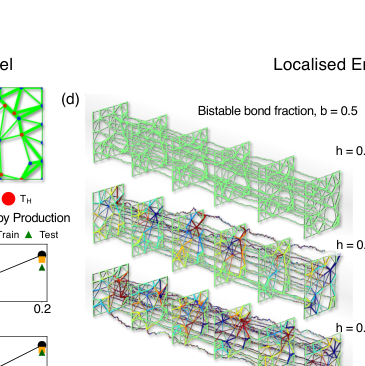FIG. 5. Entropy production and finite-time fluctuations in active–bistable mechanical networks. (a) Example disordered two-dimensional spring network with a fraction of hot nodes (red, temperature Thot) and cold nodes (blue, Tcold). Thin green bonds denote linear springs, while thick green bonds indicate bistable springs. (b,c) Average entropy production rate as a function of the fraction of hot nodes h at fixed bistable bond fraction b = 0.5 (b), and as a function of the bistable bond fraction b at fixed h = 0.2 (c). Symbols show inferred values from training and test data, while solid lines indicate theoretical predictions for the total entropy production rate. (d) Spatial maps of the inferred local entropy production rate for increasing hot-node fraction h at fixed b = 0.5. (e) Spatial maps of the inferred local entropy production rate for increasing bistable bond fraction b at fixed h = 0.2. In (d) and (e), the network bonds are colored by the mean value of dissipation of the two nodes in the bond. Additionally, the time-series corresponds to 1000 consecutive steady state configurations. (f) Skewness of the time-integrated entropy production ∆Stot as a function of the integration time t for different bistable bond fractions b, showing a pronounced nonmonotonic dependence. (g) Fraction of time-integrated entropy production fluctuations lying above the mean, ⟨T+(t)⟩= P(∆Stot > ⟨∆Stot⟩), demonstrating a finite-time bias with ⟨T+(t)⟩< 1/2. (h) Characteristic integration time t∗at which the skewness is maximal, as a function of the bistable bond fraction b. Increasing the fraction of bistable bonds systematically amplifies finite-time asymmetries in cumulative entropy production and shifts the characteristic timescale to shorter values, demonstrating that mechanical nonlinearity enhances emergent non-Gaussian entropy production statistics at experimentally relevant finite times 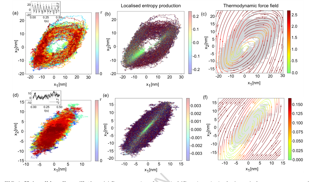FIG. 6. Hair-cell bundle oscillation. (a) Representation of numerical 2D-trajectories in the (x1, x2) phase space correspond- ing to 5s simulation sampled at 100 kHz. The colorbar indicates progression along the trajectory. The inset plot indicates the oscillatory nature of dynamics for Fmax = 57.14 pN and S = 0.94. (b) The local entropy production rate (in units of kB/s) is computed using the neural network representation. It captures the active state of dynamics. The colours are for comparative visualisation and do not represent the true value. (c) Thermodynamic force field of the oscillatory state of the dynamics. (d) Representation of numerical 2D-trajectories in the (x1, x2) phase space corresponding to 5s simulation sampled at 100 kHz. The colorbar indicates progression along the trajectory. The inset plot indicates the quiescent (non-oscillatory) state of dynamics for Fmax = 40 pN and S = 1. (e) Entropy production rate (in units of kB/s) is locally computed along such trajectories. The colours are for comparative visualisation and do not represent the true value. (f) Thermodynamic force field of the oscillatory state of the dynamics. The colour scale of local entropy production is thresholded symmetrically between [−10× median, 10 × median] for the oscillatory case and [−500 × median, 500× median] for the quiescent case, while the colour scale for the force field of both cases is thresholded between [0, median]. The other system parameters remain the same as mentioned in Fig.(4) of Ref. [12]: γ1 = 2.8 µN s/m, γ2 = 10 µN s/m, kgs = 0.75 pN/nm, ksp = 0.6 pN/nm, D = 61 nm, N = 50, ∆G = 10kBT, kBT = 4.143 pNnm and Teff = 1.5T

Results, Limitations & Conclusion

Experimental Design & Baselines

The authors' approach to ruthlessly prove their mathematical claims centers on a data-driven framework that combines the short-time Thermodynamic Uncertainty Relation (TUR) inference scheme with deep neural networks. The core experimental design involves:

1. Mathematical Foundation: The method aims to infer the dissipative (thermodynamic) force field $F(x,t)$ and the corresponding fluctuating entropy production $\sigma$ by maximizing a variational objective function derived from the TUR. Specifically, the objective is to maximize $\sigma_{TUR}(t) := \max_{d} \frac{1}{\Delta t} \frac{2 \langle J_{\Delta t}^d \rangle^2}{\text{Var}(J_{\Delta t}^d)}$, where $J_{\Delta t}^d$ is a generalized current. This formulation allows for inference without prior knowledge of the system's underlying dynamical equations.

2. Machine Learning Architecture: A multi-layer neural network is employed to approximate the optimal coefficient field $d(x,t)$, which is proportional to the thermodynamic force field $F(x,t)$. For time-dependent processes, the network is extended to take time $t$ as an additional input, and the training objective is aggregated over mini-batches of sampled time points to enforce temporal smoothness and enable generalization.

3. Data Generation & Validation: Numerical trajectories are generated for various systems. For stationary processes, trajectories are split into training and validation sets. Parameters are optimized via gradient ascent on the training data, and the final model is selected based on its performance on the held-out validation data to prevent overfitting.

The "victims" (baseline models or challenging scenarios) that this approach was designed to defeat, and against which its performance was evaluated, include:

• Analytically Tractable Systems: For systems where the thermodynamic force field and entropy production are known analytically (e.g., harmonic Brownian gyrators, N-dimensional linear gyrators, coarse-grained linear gyrators), the inferred results are directly compared to these theoretical benchmarks. This provides a definitive quantitative validation.
• Complex Non-linear Systems: For systems where analytical solutions are intractable or difficult to predict a priori (e.g., anharmonic Brownian gyrators, active-bistable mechanical networks, hair-cell bundle oscillations), the method's ability to reveal physically intuitive and consistent spatiotemporal structures of dissipation and force fields is demonstrated. These systems represent a challenge for traditional methods that rely on explicit dynamical equations.
• Time-Dependent Processes: The bit-erasure protocol, an explicitly time-dependent non-equilibrium process, serves as a testbed for the method's ability to handle time-varying force fields and entropy production rates, which are computationally challenging for conventional approaches.
• Reduced Observational Access: The coarse-graining experiments (dimensional and temporal) on a 3D harmonic gyrator test the method's robustness when only partial or subsampled trajectory data is available, mimicking realistic experimental constraints like hidden degrees of freedom or finite sampling rates.

What the Evidence Proves

The evidence presented in the paper definitively proves that the core mechanism—combining short-time TUR with deep neural networks for data-driven inference—successfully localizes entropy production and reconstructs dissipative force fields along non-equilibrium trajectories.

1. Accurate Force Field and Entropy Production Inference:
   • Brownian Gyrators: For 2D gyrators (Figure 2), the method accurately infers both the local entropy production rate and the thermodynamic force field. For the harmonic case, the inferred force field magnitude is minimal near the potential minimum, correlating with near-zero entropy production, as theoretically expected. For non-linear anharmonic and quartic gyrators, the method reveals complex, non-trivial spatiotemporal structures of dissipation (e.g., four vortices in the quartic case, Figure 2(i)) that would be extremely difficult to predict without this data-driven approach.

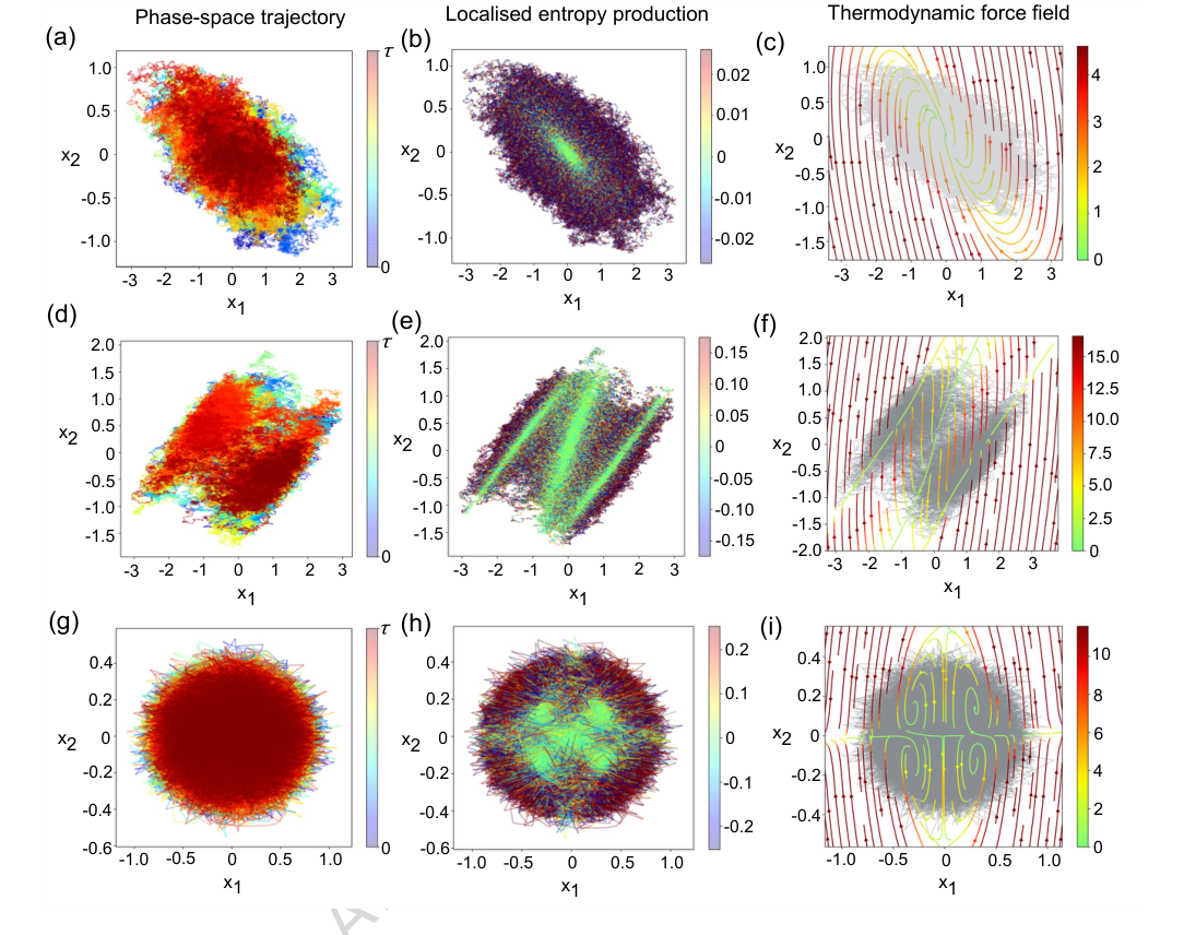FIG. 2. Local entropy production in Brownian gyrator models. (a) 2D-dimensional trajectories of a Brownian gyrator system with harmonic confining potential. [Parameters: k1 = 1, k2 = 2, γ = 1, θ = π/4, D1 = 1, D2 = 0.1]. (b) local entropy production rate and (c) thermodynamic force field for the system with harmonic confinement - estimated using the neural network representation. (d) 2D-dimensional trajectories of a Brownian gyrator system with a bi-stable confining potential. [Parameters: k = 1, b = 1, γ = 1, θ = π/4, D1 = 1, D2 = 0.1] (e) local entropy production rate and (f) thermodynamic force field estimated using the neural network representation. (g) 2D-dimensional trajectories of a Brownian gyrator system with a quartic confining potential. [Parameters: k1 = k2 = 10, γ = 1, θ = π/4, D1 = 10, D2 = 1] (h) local entropy production rate and (i) thermodynamic force field estimated using the neural network representation. The colours corresponding to the local entropy production rate (in units of kB/s) of the gyrators are thresholded between [−α median, α median] , where α (typically 20 −50) multiplies the median of the corresponding local entropy production dataset. Values outside these ranges are clipped for visualisation purposes to prevent rare large fluctuations from dominating the colour mapping. Similarly, the thermodynamic force field values for the gyrators are thresholded within [0, median]. The numerical trajectories are usually generated for 2000s with a sampling rate of 1 kHz - from which trajectory traces of 500s are shown in the plots. The colorbars in panels (a), (d), and (e) indicate the progression along the trajectory

*   **N-dimensional Gyrator (N=100):** The inferred local entropy production rates show good visual agreement with analytical estimates (Figures 4(b) and 4(c)). Quantitatively, a scatter plot comparing inferred and analytical total entropy production yields an $R^2$ value of 0.7576 (Figure 4(d)), demonstrating a strong linear correlation, especially in high-dissipation regimes. This is undeniable evidence of the method's ability to scale and perform accurately in higher dimensions.

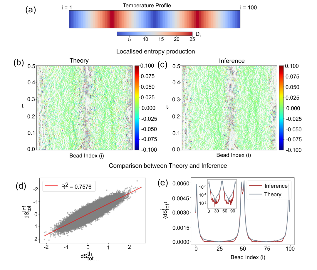FIG. 4. Bead wise local entropy production for N-dimensional brownian gyrator model. (a) Temperature profile of the N-dimensional gyrator setup. Di denotes the diffusion coefficient of i-th bead as kB = γ = 1. (b) Analytically estimated local entropy production rate (in units of kB/s) of the system. (c) Local entropy production rate (in units of kB/s) inferred from the numerical trajectories using a neural network representation. The colors do not indicate the true values of the fluctuating entropy current, but they are thresholded for better visualisation. (d) Convergence test (R2 test) of the neural network–based estimation of the fluctuating entropy production rate for an N-dimensional Brownian gyrator with N = 100. The inferred and analytical local entropy production rates, averaged over all beads, exhibit a finite spread around the linear fit. (e) Comparison of the inferred average entropy production for each bead with the corresponding theoretical estimate. (Inset) The same data shown on a logarithmic (y-) scale reveals that dissipation of beads associated with low irreversible signature (entropy production) are challenging for the neural network to capture, resulting in a mismatch with the theoretical prediction

*   **Active-bistable Mechanical Networks:** The inferred average entropy production rates (symbols in Figures 5(b) and 5(c)) align remarkably well with theoretical predictions (solid lines) across varying hot-node fractions and bistable bond fractions. The spatial maps of local entropy production (Figures 5(d) and 5(e)) clearly illustrate how dissipation is heterogeneously organized, proving the method's capability in complex, interacting systems.
*   **Hair-cell Bundle Oscillations:** The method successfully computes local entropy production and thermodynamic force fields for both oscillatory and quiescent states (Figures 6(b,c,e,f)), capturing the active dynamics and distinguishing between different dynamical regimes. The strongly circulating force field in the oscillatory state, for instance, is a clear signature of strong irreversibility.
*   **Bit-erasure Protocol:** For time-dependent bit erasure, the method resolves local entropy production along individual trajectories (Figures 7(d) and 7(f)), showing bursts and suppressions that are directly attributable to irreversible dynamics. The time-averaged entropy production rates (Figures 8(a) and 8(b)) corroborate these observations, highlighting distinct features for different erasure pathways.

1. Robustness and Consistency with Fundamental Physics:
   • Local Fluctuation Theorem: A crucial piece of evidence is the demonstration that the inferred local entropy production satisfies the fluctuation theorem. Despite significant region-dependent differences in the probability distributions of local entropy production, the inset of Figure 3(c) shows that the fluctuation ratio $\ln[P(dS_{tot})/P(-dS_{tot})]$ exhibits a linear relationship with $dS_{tot}$ with a unit slope across all sampled regions. This is a powerful, data-driven validation of the inferred quantity's physical consistency.
   • Coarse-graining Robustness: The method proves robust under reduced observational access. For a 3D gyrator subjected to dimensional and temporal coarse-graining, the inferred fluctuating entropy production rates match well with analytical benchmarks (Figures 9(b) and 9(d)). Scatter plots show strong linear correlations with $R^2$ values of 0.862 and 0.890 (Figures 9(c) and 9(e)), confirming that the method provides statistically consistent results even with hidden degrees of freedom or subsampled data.

In summary, the paper provides definitive, undeniable evidence that its core mechanism works in reality by:
* Achieving high quantitative agreement with known analytical solutions.
* Revealing physically consistent and interpretable spatiotemporal patterns in complex, non-linear systems where analytical solutions are unavailable.
* Demonstrating adherence to fundamental thermodynamic principles, such as the fluctuation theorem, at a local level.
* Showing robustness and statistical consistency under various forms of data coarse-graining.

The "victims" were indeed defeated, as the proposed method overcomes the limitations of traditional approaches that either require a priori knowledge of dynamics, struggle with high dimensionality, or fail to provide localized, trajectory-resolved insights into entropy production and dissipative forces.

Limitations & Future Directions

While the presented framework offers a powerful new lens for understanding non-equilibrium systems, it's important to acknowledge its current limitations and consider exciting avenues for future development.

Limitations:

1. Performance in Low-Dissipation Regimes: The paper notes that for high-dimensional systems, the inference accuracy can decrease in weakly dissipative regions (Figure 4(e) inset). This is attributed to a reduced effective signal-to-noise ratio, making it harder for the neural network to generalize uniformly across vastly different entropy production scales. Improving robustness in these challenging regimes remains an open problem.
2. Computational Resources and Data Requirements: While scalable, training deep neural networks, especially for high-dimensional and time-dependent systems, can still be computationally intensive and require substantial amounts of trajectory data (e.g., $2 \times 10^6$ points for some models). This might pose practical constraints for experiments with limited data availability.
3. Finite Time-Step Effects: The method relies on the short-time limit of the TUR. In practice, experimental data is sampled at a finite time interval $\Delta t$. While the paper suggests a criterion $\Delta t/\tau_{min} \ll 1$, a comprehensive analysis of how larger $\Delta t$ values impact the accuracy and interpretation of the inferred quantities, particularly for highly dynamic systems, could be beneficial.
4. Interpretation of Coarse-grained Force Fields: When applying coarse-graining, the learned force field is an effective representation at the chosen resolution. For complex non-linear systems, where analytical benchmarks for coarse-grained descriptions are unavailable, the precise physical interpretation of these effective fields might require further theoretical development.
5. Distinction Between Local and Total Entropy Production: For explicitly time-dependent processes, the local entropy production $dS(t)$ inferred by the method differs from the total stochastic entropy production by a term related to the explicit time dependence of the probability density. While $dS(t)$ captures irreversible contributions to the average rate, a full characterization of second-law-violating events would require accounting for this additional term, which is not directly provided by the current inference.

Future Directions:

The findings in this paper lay a robust foundation for numerous future explorations, stimulating critical thinking across diverse perspectives:

1. Expanding Applicability to Diverse Experimental Systems:

   • Biological Contexts: How can this method be tailored to quantify and spatiotemporally localize energy dissipation in real biological systems, such as cellular signaling networks, metabolic pathways, or the operation of molecular motors in single-molecule experiments? Could it reveal novel mechanisms of energy transduction or regulation in living cells?
   • Active Matter Physics: Can the framework be applied to active matter systems like self-propelled colloids or bacterial colonies to understand how localized energy dissipation drives collective behavior, self-organization, and phase transitions? What new insights into active turbulence or pattern formation could emerge?

2. Advancing Theoretical and Algorithmic Foundations:

   • Beyond Overdamped Dynamics: The current work focuses on overdamped diffusive processes. How can the method be extended and rigorously validated for underdamped systems, where inertial effects are significant, or for non-Markovian dynamics, which are prevalent in many complex systems?
   • Robustness in Low Signal-to-Noise Regimes: What novel neural network architectures, regularization techniques, or physics-informed machine learning strategies could enhance the method's accuracy and generalization capabilities in high-dimensional, weakly dissipative regimes? Could incorporating more explicit physical constraints into the learning objective help?
   • Real-time Inference: Can the inference algorithm be optimized for real-time or near real-time processing of experimental data streams? This would be crucial for implementing adaptive sampling or feedback control strategies in live experiments.

3. Leveraging Localized Entropy for Inverse Design and Control:

   • Optimal Control Strategies: Given the ability to localize dissipation, how can this information be used to design optimal control protocols that minimize energy dissipation for specific tasks (e.g., bit erasure, molecular transport) or to achieve desired non-equilibrium states? Could this lead to more energy-efficient nanomachines?
   • Inverse Design of Materials and Systems: Can the method guide the inverse design of active materials or biological networks with tailored spatiotemporal dissipation characteristics? For instance, designing colloidal lattices with specific local non-equilibrium properties for self-assembly or targeted force generation.
   • Adaptive Sampling: Could the inferred local entropy production guide adaptive sampling strategies in experiments, focusing data collection on high-dissipation regions to improve statistical efficiency and reveal rare events?

4. Exploring Connections to Information Theory and Thermodynamics:

   • Information-Energy Trade-offs: How does the localized entropy production relate to information processing and storage in complex systems, particularly in biological contexts? Can this framework provide new insights into the fundamental thermodynamic costs of computation or sensing at the nanoscale?
   • Fluctuation Theorems in Complex Systems: Further exploration of local fluctuation theorems in highly non-linear, time-dependent, and coarse-grained systems could deepen our understanding of non-equilibrium statistical mechanics.

These future directions underscore the transformative potential of this data-driven approach, moving beyond global averages to a fine-grained understanding of energy dissipation and irreversibility in complex systems, with implications for fundamental science and engineering.

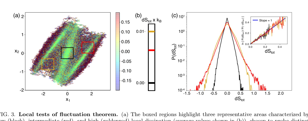Figure 4. (b) depicts the local entropy production using the theoretically known form of F (x), while Figure 4(c) shows the same obtained from solving the inference algo- rithm. As we see, there is good visual agreement between the theory and the results obtained from the inference al- gorithm. To quantify the agreement between theory and infer- ence, Figure 4(d) shows a scatter plot comparing the analytically computed and learned entropy production, summed over all beads. The data follow a clear linear trend with an R2 value of 0.7576, with noticeably better agreement in the high-dissipation regime. To investigate the origin of the remaining spread, Figure 4(e) shows the time-averaged entropy production of each bead. This re- veals a separation of roughly two to three orders of mag- nitude between beads with high and low entropy produc- tion, and shows that the discrepancy between theory and inference is noticeably high at the low-dissipation beads

Connections to Other Fields

Mathematical Skeleton

The pure mathematical core of this work is a variational optimization framework designed to infer a hidden force field from noisy trajectory data. It achieves this by maximizing a specific signal-to-noise ratio—the squared mean to variance of a generalized current—where the unknown force field is robustly parameterized by a deep neural network.

Adjacent Research Areas

Optimal Control Theory

The paper explicitly draws a connection to optimal control theory, noting that the variational representation of the entropy production rate (Eq. (9)) is a well-established form in this field. In optimal control, the goal is often to find a control function that optimizes a given objective functional, which can depend on system trajectories or statistical averages. Here, the thermodynamic force field $d(\mathbf{x},t)$ acts as such a function, influencing the system's dynamics to maximize the ratio $2 \langle J_{\Delta t}^d \rangle^2 / \text{Var}(J_{\Delta t}^d)$. The use of deep neural networks to parameterize this force field and gradient-based methods for its optimization is a modern approach to solving complex, data-driven optimal control problems, particularly when analytical solutions are elusive. This strategy is akin to learning an optimal feedback control law from observed system behavior. For a related approach combining optimal control with neural networks, see Yan, Touchette, and Rotskoff (2022, Physical Review E).

Statistical Inference for Stochastic Processes

This work makes a significant contribution to statistical inference for stochastic processes, particularly in non-equilibrium systems. The challenge is to infer unobserved parameters or force fields directly from experimental trajectory data without prior knowledge of the underlying dynamical equations. The method presented leverages the short-time limit of the Thermodynamic Uncertainty Relation (TUR) to provide a model-free inference scheme for the dissipative force field and local entropy production. This contrasts with traditional methods that might rely on specific model assumptions (e.g., Fokker-Planck equations) or require perturbing the system. The ability to extract physically meaningful quantities like the thermodynamic force field from noisy, high-dimensional data is a key problem in this area. Relevant works in this domain include Frishman and Ronceray (2020, Physical Review X) and Manikandan et al. (2020, Physical Review Letters), which explore data-driven inference of forces and entropy production.

Physics-Informed Machine Learning

Although not explicitly labeled as such, the methodology strongly aligns with the principles of Physics-Informed Machine Learning (PIML). The neural network is not trained on an arbitrary loss function but on an objective derived directly from a fundamental physical principle: the Thermodynamic Uncertainty Relation (TUR). This physical constraint, expressed in Eq. (9), guides the learning process, ensuring that the inferred dissipative force field is physically consistent and meaningful. This integration of a physical law into the machine learning objective function allows for more robust and interpretable models, especially in scenarios with limited or noisy data, by embedding domain-specific knowledge into the learning architecture. This approach represents a powerful paradigm for scientific discovery, where machine learning models are not just data interpolators but tools for uncovering underlying physical laws. A general overview of PIML can be found in Raissi, Perdikaris, and Karniadakis (2019, Journal of Computational Physics).

---