How Spurious Features are Memorized: Precise Analysis for Random and NTK Features
This paper offers a theoretical explanation for why AI models memorize irrelevant data, revealing how model stability and feature alignment play key roles.
Background & Academic Lineage
The Origin & Academic Lineage
The problem of deep learning models memorizing spurious features is a significant and well-documented phenomenon in the field, yet a rigorous theoretical framework to precisely quantify it has been largely absent. This issue arises because neural networks often learn from features in the training data that are not inherently relevant to the intended task. This can occur due to positive spurious correlations between certain patterns and the learning task (Geirhos et al., 2020; Xiao et al., 2021), or even when these patterns are rare (Yang et al., 2022) or simply irrelevant (Hermann & Lampinen, 2020). Such memorization leads to models learning spurious relationships, impacting their robustness to distribution shifts (Geirhos et al., 2019; Zhou et al., 2021), fairness (Zliobaite, 2015), and data privacy (Leino & Fredrikson, 2020).
Historically, empirical efforts have focused on mitigating this phenomenon (Plumb et al., 2022; Chang et al., 2021). However, avoiding memorization isn't always feasible, as it can sometimes be optimal for accuracy in over-parameterized models, which often achieve their best performance when trained to zero training error (Nakkiran et al., 2020; Feldman, 2020). Previous theoretical work has characterized related concepts like benign overfitting (Belkin, 2021; Bartlett et al., 2020) and in-distribution generalization of interpolating models such as random features and neural tangent kernels (Mei & Montanari, 2022; Ghorbani et al., 2021; Montanari & Zhong, 2022).
The fundamental limitation, or "pain point," of these previous approaches is that they typically model noise as residing in the labels, rather than in the input data itself. Consequently, this powerful theoretical machinery does not directly cover the memorization of spurious features embedded within the input. While practical research has explored the impact of spurious features and attempted to disentangle them from core features (Hermann & Lampinen, 2020; Singla & Feizi, 2022), theoretical analyses have predominantly focused on how learning is affected by feature complexity (Qiu et al., 2023) or the degree of overparameterization (Sagawa et al., 2020), often without fully capturing the role of the model's architecture. This paper aims to bridge this gap by providing an analytically tractable framework to understand and quantify the memorization of spurious features, specifically when they are uncorrelated with the true label of the sample.
The most precise origin of the problem of memorizing spurious features in deep learning can be traced to the empirical observations of deep learning models overfitting to training data, particularly in over-parameterized regimes. While deep learning achieved remarkable success, researchers began to notice undesirable behaviors where models would learn patterns that were correlated with the task but not causally related, or even completely irrelevant patterns.
The "why" behind its emergence is multi-faceted:
1. Over-parameterization: Modern deep learning models often have far more parameters than training data points. This capacity allows them to achieve zero training error, but also enables them to "memorize" the training data, including irrelevant details. Nakkiran et al. (2020) and Feldman (2020) highlighted that achieving zero training error often requires long training times, which can lead to memorization.
2. Spurious Correlations in Data: Real-world datasets often contain features that are statistically correlated with the true label but are not causally linked. For instance, if all images of "cats" in a dataset happen to have a specific "blue background," a model might learn to associate "blue background" with "cat" (Geirhos et al., 2020; Xiao et al., 2021). This is particularly problematic when these spurious correlations are not predictive of the true sampling distribution.
3. Irrelevant or Rare Patterns: The problem also emerges even when spurious patterns are rare or simply irrelevant to the task (Yang et al., 2022; Hermann & Lampinen, 2020). Models can still pick up on these patterns, leading to memorization.
4. Consequences for Robustness, Fairness, and Privacy: The practical implications of this memorization—such as poor out-of-distribution robustness (Geirhos et al., 2019; Zhou et al., 2021), biased predictions affecting fairness (Zliobaite, 2015), and potential data privacy breaches through information extraction (Leino & Fredrikson, 2020)—highlighted the urgent need for a deeper understanding.
The historical context shows a progression from empirical observations of overfitting to a recognition that this overfitting often involves "spurious features" rather than just random noise. The academic field then sought to move beyond qualitative descriptions and empirical mitigation strategies towards a rigorous theoretical framework.
The fundamental limitation or "pain point" of previous approaches that forced the authors to write this paper is the lack of a precise theoretical framework to quantify the memorization of spurious features when they are embedded in the input data, rather than being modeled as noise in the labels.
Previous bodies of work, while powerful, primarily focused on:
* Benign Overfitting: Characterizing models that overfit the training data but still generalize well on in-distribution test data (Belkin, 2021; Bartlett et al., 2020).
* In-distribution Generalization: Analyzing interpolating models like Random Features (RF) and Neural Tangent Kernels (NTK) where noise is typically assumed to be in the labels, not in the input features (Mei & Montanari, 2022; Ghorbani et al., 2021).
The crucial gap was that these theoretical tools "do not cover the memorization of spurious features, as noise is generally modelled to be in the labels, rather than in the input data." Furthermore, while practical work attempted to understand and disentangle spurious features, theoretical approaches remained largely focused on feature complexity or over-parameterization, "without capturing the role of the architecture." This paper directly addresses this pain point by providing an analytically tractable framework to understand and quantify spurious feature memorization, explicitly considering the model's architecture and activation function.
Intuitive Domain Terms
To make complex concepts accessible to a zero-base reader, let's break down some highly specialized terms using everyday analogies:
- Spurious Features ($y$): Imagine you're teaching a smart robot to identify "apples" in photos. The "core feature" is the apple itself (its shape, color, stem). A "spurious feature" might be the specific kitchen counter where all your training photos of apples were taken. The counter is present in the photos, but it has nothing to do with what makes an apple an apple.
- Memorization (of spurious features): This occurs when the robot, instead of just learning about apples, also "remembers" the kitchen counter. If you later show it an apple on a different surface, it might hesitate or even fail to recognize it because it has mistakenly associated "kitchen counter" with "apple-ness." The robot has "memorized" an irrelevant detail.
- Feature Alignment ($F_\phi(z^s, z)$): This measures how similar the "irrelevant part" (just the kitchen counter, $z^s$) looks to the "whole picture" (the apple on the kitchen counter, $z$) from the robot's internal processing perspective. If the robot's visual system heavily processes backgrounds, then seeing just the kitchen counter might strongly "align" with its memory of an apple on that counter.
- Stability ($S_{z_1}$): This refers to how much the robot's overall understanding of apples changes if you add or remove one specific training photo (e.g., one apple on the kitchen counter). A "stable" robot's knowledge won't drastically change. If the robot's "kitchen counter = apple" belief is very unstable, removing just one photo might make it completely drop the association. If it's stable, it will retain the belief even with minor changes to its training examples.
Notation Table
| Notation | Description |
|---|---|
| $z = [x, y]$ | An input sample, decomposed into a core feature $x$ and a spurious feature $y$. |
| $x$ | The core feature of a sample, relevant to the true label. |
| $y$ | The spurious feature of a sample, uncorrelated with the true label. |
| $g(x)$ | The true label, which depends only on the core feature $x$. |
| $z^s = [-, y]$ | A "spurious counterpart" of a sample, where the core feature $x$ is removed (e.g., replaced with zeros), leaving only the spurious feature $y$. |
| $f(z, \theta^*)$ | The model's prediction function for input $z$ with optimal parameters $\theta^*$. |
| $\phi(z)$ | The feature map (or feature vector) of an input $z$, transforming raw data into a higher-dimensional representation. |
| $\theta^*$ | The optimal parameters of the model, learned from the full training dataset. |
| $\theta^*_{-1}$ | The optimal parameters of the model, learned from the training dataset excluding sample $z_1$. |
| $S_{z_1}$ | Stability of the model with respect to training sample $z_1$, measuring the change in output when $z_1$ is removed. |
| $F_\phi(z, z_1)$ | Feature alignment between samples $z$ and $z_1$ in the feature space induced by $\phi$. |
| $P_{\Phi_{-1}}$ | The projector onto the span of the rows of the feature matrix $\Phi_{-1}$ (all training samples except $z_1$). |
| $R_{Z_{-1}}$ | Generalization error of the model trained on the dataset $Z_{-1}$ (excluding $z_1$). |
| $\gamma_\phi$ | A proportionality constant related to feature alignment, dependent on the feature map $\phi$ and activation function. |
| $\alpha = d_y/d$ | The fraction of the input dimension attributed to the spurious feature. |
| $h_i$ | The $i$-th Hermite polynomial, used to characterize activation functions. |
| $N$ | The number of training samples. |
| $k$ | The number of neurons (for RF) or width (for NTK). |
| $d$ | The total input dimension. |
| $d_x$ | Dimension of the core feature $x$. |
| $d_y$ | Dimension of the spurious feature $y$. |
| RF | Random Features model. |
| NTK | Neural Tangent Kernel model. |
Problem Definition & Constraints
Core Problem Formulation & The Dilemma
Deep learning models, particularly over-parameterized ones, are known to memorize "spurious features" present in their training data. These features are patterns or attributes that are uncorrelated with the true label of a sample but might co-occur with it in the training set. For instance, if a model is trained to identify cats, and all training images of cats happen to have a specific background (the spurious feature), the model might learn to associate the background with the "cat" label, rather than the cat itself.
The core problem this paper addresses is the lack of a rigorous theoretical framework to precisely quantify and understand how these spurious features are memorized. Previous theoretical work has largely focused on "benign overfitting," where noise is modeled in the labels, or on the complexity of features and over-parameterization, without specifically addressing spurious features embedded within the input data or the role of model architecture.
Input/Current State: We start with deep learning models trained on datasets where each sample $z$ is composed of a core feature $x$ and a spurious feature $y$, formally $z = [x, y]$. The true label $g$ for a sample $z_i$ is $g_i = g(x_i)$, meaning it depends only on the core feature $x_i$ and is independent of the spurious feature $y_i$. These models are typically over-parameterized and trained until they achieve zero training error, meaning they perfectly fit the training data. Formally, we model the sample $z$ as composed by two distinct parts, i.e., $z = [x, y]$, where $x$ is the core feature and $y$ the spurious one, see Figure 1 for an illustration. The memorization of spurious features is captured by the correlation between the true label $g$ of the training sample and the output of the model evaluated on the spurious sample $z^s = [-, y]$, where "-" corresponds to removing the core feature $x$ (e.g., replacing it with all zeros).
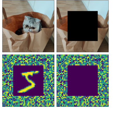 Figure 1. Example of a training sample z (top-left) and its spuri- ous counterpart zs (top-right). In experiments, we add a noise background (y) around the original images (x) before training (bottom-left). We then query the trained model only with the noise component (bottom-right)
Output/Goal State: The desired outcome is an analytically tractable framework that can precisely characterize the memorization of spurious features. This involves:
1. Quantifying the extent of memorization using a metric like the covariance between the true label $g_i$ and the model's output when queried with a "spurious counterpart" of the sample, $z_i^s = [x, y_i]$ (where $x$ is replaced by an independent feature, e.g., all zeros).
2. Decomposing this memorization into two key components: the model's stability with respect to individual training samples and a novel concept called "feature alignment" between the original and spurious samples.
3. Unveiling how model choices (like Random Features or Neural Tangent Kernel architectures) and activation functions influence this feature alignment and, consequently, the memorization of spurious features.
4. Ultimately, the goal is to provide insights that enable the design of machine learning models that are less prone to memorizing spurious correlations, thereby improving robustness to distribution shifts, fairness, and data privacy.
The Dilemma: The painful trade-off that has trapped previous researchers, and which this paper seeks to navigate, is that avoiding the memorization of spurious features is often at odds with achieving high accuracy. Over-parameterized deep learning models, which are prevalent today, frequently achieve their best performance when trained long enough to reach zero training error. This process of perfectly fitting the training data often entails memorizing spurious correlations, as it's an "easy" way for the model to reduce training loss. Therefore, improving one aspect (reducing spurious memorization) typically risks degrading another (overall training accuracy or generalization on core features), creating a difficult balancing act.
Constraints & Failure Modes
The problem of theoretically quantifying spurious feature memorization in deep learning is inherently challenging due to several harsh, realistic constraints:
- Computational and Theoretical Tractability: Full deep neural networks are notoriously complex, making their theoretical analysis extremely difficult. The paper addresses this by focusing on two simplified yet powerful theoretical models: Random Features (RF) and Neural Tangent Kernel (NTK) regression. These models are chosen because they are "analytically tractable" and "widely analyzed in the theoretical literature," allowing for precise mathematical characterization. This implies that extending the exact analytical results to arbitrary, complex deep learning architectures remains a significant hurdle.
- Specific Definition of Spurious Features: The analysis is strictly confined to spurious features that are uncorrelated with the true learning task. If spurious features were correlated, the problem would shift from pure "memorization" to "shortcut learning" or "spurious correlation exploitation," which requires a different theoretical treatment. This is a crucial boundary condition for the current framework.
- Data Distribution Assumptions: The theoretical results rely on specific assumptions about the data distribution. For instance, input samples $z_i = [x_i, y_i]$ are assumed to be independently and identically distributed (i.i.d.) from a product distribution $P_z = P_x \times P_y$, meaning core features $x_i$ and spurious features $y_i$ are independent. Furthermore, specific properties like zero mean and controlled $L_2$ norms ($||x||_2 = \sqrt{d_x}$, $||y||_2 = \sqrt{d_y}$) are assumed for $x$ and $y$. Both $P_x$ and $P_y$ must satisfy Lipschitz concentration. These assumptions simplify the analysis but might not hold universally for all real-world datasets.
- Over-parameterization and High-Dimensionality Assumptions: The framework operates within specific regimes of over-parameterization and high-dimensionality. For RF models, conditions like $N \log^3 N = o(k)$, $\sqrt{d} \log d = o(k)$, and $k \log^4 k = o(d^2)$ are required, implying a large number of neurons $k$ relative to data points $N$ and input dimension $d$. For NTK models, the conditions are $N \log^3 N = o(kd)$, $N > d$, and $k = O(d)$. These conditions are essential for ensuring kernel invertibility and the model's ability to interpolate the data, but they define a specific operational regime.
- Activation Function Properties: The activation function $\phi$ (or its derivative $\phi'$ for NTK) is assumed to be non-linear and L-Lipschitz. These properties are critical for the mathematical derivations, particularly those involving Hermite coefficients and concentration inequalities.
- Kernel Invertibility: A fundamental constraint for the generalized linear regression model used is that the induced kernel $K$ on the training set must be invertible. This ensures that the model can perfectly fit any set of labels $G$ and that the Moore-Penrose inverse, used in the solution for the optimal parameters $\theta^*$, is well-defined.
- Generalization to Real-World Scenarios: While the paper provides numerical experiments on standard datasets (MNIST, CIFAR-10) and different neural network architectures (fully connected, convolutional, ResNet) to show that theoretical predictions transfer, the analytical proofs are primarily for simplified models and synthetic data. Bridging this gap with full theoretical rigor for complex, real-world deep learning systems remains an an open challenge. The current analysis is a significant step but does not fully encompass the vast diversity of practical deep learning setups.
Why This Approach
The Inevitability of the Choice
The selection of Random Features (RF) and Neural Tangent Kernel (NTK) regression models was not arbitrary but rather a strategic necessity driven by the specific theoretical gap this paper aims to bridge. The core problem is to understand and quantifiy the memorization of spurious features that are uncorrelated with the true learning task, where these features manifest as noise within the input data itself, not just in the labels.
Existing theoretical frameworks, even those leveraging powerful tools like RF and NTK for phenomena such as benign overfitting or in-distribution generalization, predominantly model noise as residing in the labels. This fundamental difference meant that while these models (RF and NTK) were theoretically appealing for their analytical tractibility, their established theoretical machinery did not directly address the input-level spurious feature memorization problem. The authors realized that traditional "SOTA" methods, often empirical in nature (e.g., standard CNNs, Diffusion models, or Transformers), while powerful for practical tasks, lacked the analytical transparency required for a precise, quantifiable theoretical characterization of this specific memorization phenomenon. Therefore, extending the theoretical understanding of RF and NTK, known for their analytical tractability in related learning theory, became the only viable path to develop the rigorous framework needed.
Comparative Superiority
This method offers qualitative superiority not merely through performance metrics, but by providing an unprecedented structural advantage in theoretical understanding. The paper introduces a novel concept: "feature alignment" ($F_\phi(z, z_1)$), which quantifies the similarity in feature space between a training sample and its spurious counterpart. This, combined with the classical notion of model stability ($S_{z_1}$), forms a two-pronged approach to precisely characterize how spurious features are memorized.
The structural advantage lies in the analytical tractability of RF and NTK models within this framework. They allow for closed-form expressions for the proportionality constant ($\gamma_\phi$) that links memorization to generalization error. This level of mathematical interpretability is overwhelmingly superior to previous empirical gold standards, which often provide performance gains without deep insight into the underlying memorization mechanisms. While the method doesn't reduce memory complexity from $O(N^2)$ to $O(N)$ or explicitly handle high-dimensional noise better in a computational sense, it provides a quantifiable measure of how spurious features (modeled as input noise) are memorized, unveiling the crucial role of the model architecture and its activation function in this process.
Alignment with Constraints
The chosen approach perfectly aligns with the problem's harsh requirements by leveraging the unique properties of Random Features and Neural Tangent Kernels. The primary constraint was to develop an analytically tractable framework to quantify the memorization of spurious features that are uncorrelated with the true label and embedded in the input data.
The generalized linear regression setting, combined with RF and NTK models, provides exactly this analytical tractability. The formal decomposition of a sample $z$ into core feature $x$ and spurious feature $y$ ($z = [x, y]$), where $y$ is independent of the true label $g(x)$, directly mirrors the problem definition. The framework's ability to precisely characterize memorization through stability and the novel feature alignment term allows for a direct quantification of the phenomenon. Furthermore, the assumptions made (e.g., data distribution, over-parameterization, activation function properties) are carefully chosen to ensure that the mathematical analysis remains feasible and yields meaningful, closed-form expressions, thereby creating a perfect "marriage" between the problem's theoretical demands and the solution's analytical capabilities.
Rejection of Alternatives
The paper does not explicitly "reject" other popular deep learning architectures like GANs or Diffusion models in the sense of deeming them inferior for all tasks. Instead, the implicit rejection stems from their current lack of a rigorous, analytically tractable theoretical framework for precisely quantifying spurious feature memorization in the input data.
The authors highlight that while practical work has explored spurious features, these approaches often fail to capture the role of the architecture or provide a quantifiable theoretical understanding. Existing theoretical machinery for models like RF and NTK, when applied to problems like benign overfitting, typically models noise in the labels, not as spurious features in the input. This means that while these models (RF/NTK) themselves are powerful, their existing theoretical analysis was insufficient for the specific problem at hand. The paper's contribution is to extend this theoretical analysis for RF and NTK to cover spurious feature memorization, rather than to propose an entirely new model. Therefore, the "rejection" is not of the models themselves, but of the insufficiency of current theoretical tools to provide the deep, quantifiable insights that this paper seeks for the specific problem of input-level spurious feature memorization.
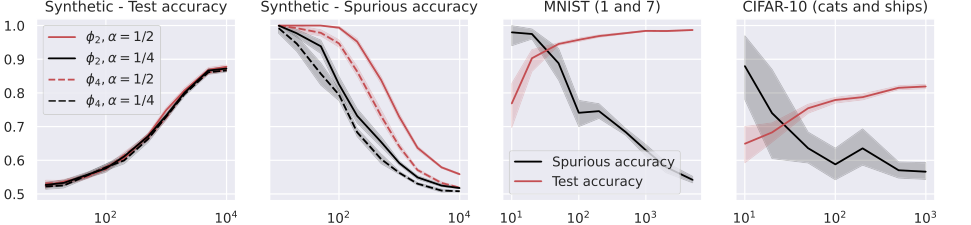 Figure 6. Test and spurious accuracies as a function of the number of training samples N, for various binary classification tasks. In the first two plots, we consider the NTK model in (24) with k = 100 trained over Gaussian data with d = 1000. The labeling function is g(x) = sign(u⊤x). We repeat the experiments for α = {0.25, 0.5}, and for the two activations whose derivatives are ϕ′ 2 = h0 + h1 and ϕ′ 4 = h0 + h3, where hi denotes the i-th Hermite polynomial (see Appendix A.1). In the last two plots, we consider the same model with ReLU activation, trained over two MNIST and CIFAR-10 classes. The width of the noise background is 10 pixels for MNIST and 8 pixels for CIFAR-10, see Figure 1. The spurious accuracy is obtained by querying the model only with the noise background from the training set, replacing all the other pixels with 0, and taking the sign of the output. As we consider binary classification, an accuracy of 0.5 is achieved by random guessing. We plot the average over 10 independent trials and the confidence band at 1 standard deviation
Mathematical & Logical Mechanism
The Master Equation
The paper's core mechanism for understanding how spurious features are memorized hinges on three interconnected mathematical definitions: the model's stability, the feature alignment between samples, and the relationship that ties them together. These equations collectively describe the sensitivity of a trained model to individual training points and how this sensitivity is modulated by the similarity of features in the model's internal representation space.
First, the stability of the model with respect to a training sample $z_1$ is defined as:
$$S_{z_1} := f(\cdot, \theta^*) - f(\cdot, \theta^*_{-1}) \quad (5)$$
This quantity measures how much the model's output changes when a specific training sample $z_1$ is either included or excluded from the training dataset.
Second, the feature alignment between two samples, $z$ and $z_1$, in the feature space induced by the feature map $\phi$ is given by:
$$F_\phi(z, z_1) := \frac{\phi(z)^\top P_{\Phi_{-1}} \phi(z_1)}{\|P_{\Phi_{-1}}\phi(z_1)\|_2^2} \quad (8)$$
This term quantifies the similarity or "alignment" of the feature representation of a generic sample $z$ with that of a specific training sample $z_1$, after projecting onto a subspace defined by the rest of the training data.
Finally, the crucial link between stability and feature alignment is established by Lemma 4.1, which states:
$$S_{z_1}(z) = F_\phi(z, z_1) S_{z_1}(z_1) \quad (9)$$
This equation reveals that the stability of the model's output for any sample $z$ (when $z_1$ is removed) is directly proportional to the stability at $z_1$ itself, scaled by their feature alignment. This elegant relationship forms the bedrock of the paper's analysis of memorization.
Term-by-Term Autopsy
Let's dissect each component of these master equations to understand their precise mathematical definition, their physical or logical role in the model, and the rationale behind the chosen mathematical operations.
Equation (5): Stability $S_{z_1}$
* $S_{z_1}$: This symbol represents the stability of the model with respect to the training sample $z_1$.
* Mathematical Definition: A scalar value representing the difference in model predictions.
* Physical/Logical Role: It quantifies the influence of a single training sample $z_1$ on the model's output. A large $S_{z_1}$ means that removing $z_1$ significantly alters the model's predictions, indicating that $z_1$ is "memorized" or has a strong impact.
* $f(\cdot, \theta^*)$: This is the prediction function of the model trained on the full dataset.
* Mathematical Definition: $f(z, \theta^*) = \phi(z)\theta^*$, where $\phi(z)$ is the feature vector for input $z$ and $\theta^*$ are the optimal parameters learned from the entire training set $Z$.
* Physical/Logical Role: Represents the model's output when all available training data has been used to learn its parameters.
* $f(\cdot, \theta^*_{-1})$: This is the prediction function of the model trained on the dataset without $z_1$.
* Mathematical Definition: $f(z, \theta^*_{-1}) = \phi(z)\theta^*_{-1}$, where $\theta^*_{-1}$ are the optimal parameters learned from the training set $Z_{-1}$ (which is $Z$ excluding $z_1$).
* Physical/Logical Role: Represents the model's output when a specific training sample $z_1$ has been omitted from the training process.
* $- (subtraction)$:
* Why used: Subtraction is used to directly measure the change or difference in the model's output due to the presence or absence of $z_1$. This is a standard way to quantify influence or sensitivity. If multiplication were used, it would measure a ratio, which is not the desired metric for "change."
Equation (8): Feature Alignment $F_\phi(z, z_1)$
* $F_\phi(z, z_1)$: This symbol denotes the feature alignment between sample $z$ and training sample $z_1$.
* Mathematical Definition: A scalar value representing a normalized projection.
* Physical/Logical Role: It measures how "similar" the feature representation of a generic sample $z$ is to that of a specific training sample $z_1$, within the feature space. This similarity is crucial because it indicates how much information about $z_1$ might be "transferred" or "aligned" with $z$ in the model's internal representation.
* $\phi(z)$: The feature map of an input sample $z$.
* Mathematical Definition: A vector $\phi(z) \in \mathbb{R}^p$ obtained by applying a feature map function $\phi: \mathbb{R}^d \to \mathbb{R}^p$ to the input $z \in \mathbb{R}^d$.
* Physical/Logical Role: This transforms the raw input data $z$ into a higher-dimensional feature representation that the linear model operates on. It's the model's internal "understanding" of the input.
* $\phi(z_1)$: The feature map of the training sample $z_1$.
* Mathematical Definition: Similar to $\phi(z)$, but for the specific training sample $z_1$.
* Physical/Logical Role: Represents the model's internal feature representation of the training sample whose influence is being studied.
* $P_{\Phi_{-1}}$: The projector onto the span of the rows of $\Phi_{-1}$.
* Mathematical Definition: A projection matrix $P_{\Phi_{-1}} \in \mathbb{R}^{p \times p}$ such that $P_{\Phi_{-1}} = \Phi_{-1}^\top (\Phi_{-1}\Phi_{-1}^\top)^{-1} \Phi_{-1}$ (if $\Phi_{-1}\Phi_{-1}^\top$ is invertible). It projects vectors onto the row space of $\Phi_{-1}$.
* Physical/Logical Role: This projector effectively "filters out" or "normalizes" the feature vectors by considering the subspace spanned by the features of all other training samples (excluding $z_1$). This ensures that the alignment is measured relative to the collective information from the rest of the dataset, making it a more robust measure of unique alignment.
* $\top (transpose)$:
* Why used: The transpose is used to perform an inner product (dot product) between two vectors, $\phi(z)$ and $P_{\Phi_{-1}}\phi(z_1)$. This operation quantifies the linear correlation or similarity between the two feature vectors.
* $\cdot$ (multiplication):
* Why used: Matrix-vector multiplication (e.g., $P_{\Phi_{-1}}\phi(z_1)$) applies the linear transformation defined by the projector. Vector-vector multiplication (dot product) quantifies similarity.
* $\|\cdot\|_2^2$: The squared L2 norm.
* Mathematical Definition: For a vector $v$, $\|v\|_2^2 = v^\top v = \sum_i v_i^2$.
* Physical/Logical Role: This term in the denominator normalizes the alignment. It ensures that $F_\phi(z, z_1)$ is a measure of relative alignment, making it invariant to the scale of the feature vectors themselves. It essentially measures the cosine similarity (or a related projection) in the feature space.
* $/ (division)$:
* Why used: Division by the squared L2 norm is a normalization step, common in defining projections or similarities, ensuring the alignment metric is properly scaled.
Equation (9): Relationship $S_{z_1}(z) = F_\phi(z, z_1) S_{z_1}(z_1)$
* $S_{z_1}(z)$: The stability of the model's output at a generic sample $z$.
* Mathematical Definition: $f(z, \theta^*) - f(z, \theta^*_{-1})$.
* Physical/Logical Role: This is the specific change in the model's prediction for sample $z$ when $z_1$ is removed.
* $S_{z_1}(z_1)$: The stability of the model's output at the training sample $z_1$ itself.
* Mathematical Definition: $f(z_1, \theta^*) - f(z_1, \theta^*_{-1})$.
* Physical/Logical Role: This represents the direct impact of $z_1$ on its own prediction. If the model perfectly interpolates, $f(z_1, \theta^*) = g_1$, so $S_{z_1}(z_1) = g_1 - f(z_1, \theta^*_{-1})$. This term captures how well the model learns $z_1$'s label when $z_1$ is present, compared to when it's absent.
* $\cdot$ (multiplication):
* Why used: Multiplication is used to show a direct proportionality. The change in prediction for $z$ is a scaled version of the change for $z_1$, where the scaling factor is the feature alignment. This implies a linear relationship: if $z$ is highly aligned with $z_1$ in feature space, then removing $z_1$ will affect $z$'s prediction similarly to how it affects $z_1$'s prediction.
Step-by-Step Flow
Imagine a data point $z$ entering this mathematical engine, along with a specific training sample $z_1$ and its spurious counterpart $z^s$. The goal is to understand how the model's output for $z^s$ might be influenced by $z_1$, indicating memorization.
- Feature Extraction: First, the raw input $z$ and the specific training sample $z_1$ are fed into the model's feature map $\phi$. This transforms them into their internal feature representations, $\phi(z)$ and $\phi(z_1)$, respectively. Think of this as the initial processing unit, converting raw data into a format the model can "understand."
- Subspace Projection: Next, $\phi(z_1)$ is projected onto the subspace spanned by the features of all other training samples, $\Phi_{-1}$, using the projector $P_{\Phi_{-1}}$. This step isolates the unique contribution of $z_1$'s features, relative to the rest of the training data.
- Feature Alignment Calculation: The projected $\phi(z_1)$ is then compared with $\phi(z)$ via an inner product, and normalized by the magnitude of the projected $\phi(z_1)$. This computes $F_\phi(z, z_1)$, the feature alignment. This unit determines how "similar" $z$ is to $z_1$ in the model's feature space, after accounting for the background of other training data.
- Model Training (Implicit): In parallel, two versions of the model are "trained." One, $f(\cdot, \theta^*)$, uses the entire training dataset $Z$ (including $z_1$). The other, $f(\cdot, \theta^*_{-1})$, uses the dataset $Z_{-1}$ (excluding $z_1$). The parameters $\theta^*$ and $\theta^*_{-1}$ are derived from these training processes.
- Stability Measurement at $z_1$: The model's output for $z_1$ is computed using both sets of parameters: $f(z_1, \theta^*)$ and $f(z_1, \theta^*_{-1})$. The difference between these two outputs, $S_{z_1}(z_1) = f(z_1, \theta^*) - f(z_1, \theta^*_{-1})$, is calculated. This unit measures how much $z_1$ itself changes the model's prediction for $z_1$. If the model perfectly interpolates, $f(z_1, \theta^*) = g_1$, so this term becomes $g_1 - f(z_1, \theta^*_{-1})$, representing the "memorization" of $z_1$'s label.
- Propagating Stability: Now, the feature alignment $F_\phi(z, z_1)$ and the stability at $z_1$, $S_{z_1}(z_1)$, are multiplied together to yield $S_{z_1}(z) = F_\phi(z, z_1) S_{z_1}(z_1)$. This means the influence of $z_1$ on a generic sample $z$ is directly proportional to how aligned $z$ is with $z_1$ in feature space, scaled by $z_1$'s own impact.
- Quantifying Memorization: Finally, to quantify the memorization of spurious features, the paper considers the covariance
Cov(f(z^s, θ*), g_i). This involves evaluating the model on a spurious sample $z^s = [-, y]$ (where the core feature $x$ is removed or zeroed out, leaving only the spurious feature $y$) and correlating its output with the true label $g_i$ (which only depends on $x_i$). The derived relationship (Equation 11) shows that this covariance is bounded by $\gamma_\phi \sqrt{R_{Z_{-1}}} \sqrt{\text{Var}(g_i)}$, where $\gamma_\phi$ is a constant related to feature alignment and $R_{Z_{-1}}$ is the generalization error. This final step connects the mechanical assembly line of feature processing and stability to the ultimate measure of spurious feature memorization.
Optimization Dynamics
The paper operates within the framework of generalized linear regression, where the model parameters $\theta$ are learned by minimizing an empirical risk with a quadratic loss, as shown in Equation (2): $\min_\theta \| \Phi \theta - G \|_2^2$. In this setting, the optimization process leads to a closed-form solution for the optimal parameters $\theta^*$, given by Equation (3): $\theta^* = \theta_0 + \Phi^+(G - f(Z, \theta_0))$.
This means the "learning" or "optimization dynamics" are not about an iterative gradient descent process exploring a complex loss landscape in the traditional sense, but rather about the properties of this direct, interpolating solution. The paper explicitly states that "gradient descent converges to the interpolator which is the closest in l2 norm to the initialization." This implies that the model is trained to achieve zero training error, a characteristic of over-parameterized models.
The key "dynamics" analyzed here are:
1. Interpolation: The model's ability to perfectly fit the training data (achieving zero training error) is a direct consequence of the over-parameterized regime and the chosen optimization objective. This interpolation is what allows for the memorization of spurious features.
2. Generalization Error's Role: The paper's main result (Equation 11) shows that the memorization of spurious features (quantified by Cov(f(z^s, θ*), g_i)) is directly proportional to the generalization error $R_{Z_{-1}}$. This means that as the model's ability to generalize to unseen data improves (i.e., $R_{Z_{-1}}$ decreases), its tendency to memorize spurious features also weakens. This is a crucial insight into the behavior of the interpolating solution.
3. Feature Alignment's Influence: The proportionality constant $\gamma_\phi$ in the memorization bound (Equation 11) is derived from the feature alignment $F_\phi(z_1, z_1)$. This constant, which depends on the feature map $\phi$ and the activation function, shapes the "loss landscape" in a way that dictates how strongly spurious features are memorized even when the model generalizes well. A higher $\gamma_\phi$ implies greater memorization for a given generalization error. The paper's analysis of RF and NTK models precisely characterizes this $\gamma_\phi$, revealing how the model architecture and activation function influence the memorization dynamics.
4. Stability as a Proxy: The stability $S_{z_1}(z_1)$ acts as a measure of how much the model relies on individual training points to achieve interpolation. If $S_{z_1}(z_1)$ is large, the model is highly sensitive to $z_1$, indicating that $z_1$ is strongly "memorized." The optimization process, by finding an interpolating solution, inherently creates this stability, which then propagates through feature alignment to influence spurious memorization.
In essence, the "optimization dynamics" are understood through the lens of the characteristics of the interpolating solution $\theta^*$ rather than the iterative steps of finding it. The model learns to perfectly fit the data, and the paper analyzes the inherent trade-offs and consequences of this learning strategy, particularly concerning the memorization of irrelevant information. The gradients, while leading to $\theta^*$, are not explicitly analyzed in their iterative behavior but rather their final state's properties.
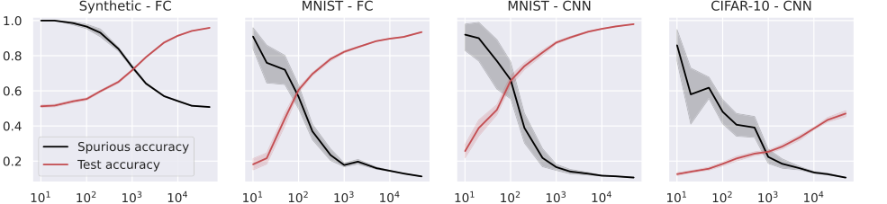 Figure 4. Test and spurious accuracies as a function of the number of training samples N, for a fully connected (FC, first two plots), and a small convolutional neural network (CNN, last two plots). In the first plot, we use synthetic (Gaussian) data with d = 1000, and the labeling function is g(x) = sign(u⊤x). As we consider binary classification, the accuracy of random guessing is 0.5. The other plots use subsets of the MNIST and CIFAR-10 datasets, with an external layer of noise added to images, see Figure 1. As we consider 10 classes, the accuracy of random guessing is 0.1. We plot the average over 10 independent trials and the confidence band at 1 standard deviation
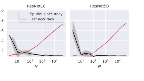 Figure 5. Test and spurious accuracies as a function of the number of training samples N, for two ResNet architectures. We use subsets of the CIFAR-10 dataset, with an external layer of noise added to images, see Figure 1. As we consider 10 classes, the accuracy of random guessing is 0.1. We plot the average over 10 independent trials and the confidence band at 1 standard deviation
Results, Limitations & Conclusion
Experimental Design & Baselines
To rigorously validate their theoretical claims, the authors meticulously designed a series of experiments, pitting their mathematical predictions against empirical observations across various model types and datasets. The core idea was to create scenarios where spurious features—irrelevant noise or background information—were present in the training data but not predictive of the true label. Then, they measured how much the models "memorized" these irrelevant features.
The "victims" in these experiments were not alternative models in the traditional sense, but rather the very Random Features (RF) and Neural Tangent Kernel (NTK) models under investigation, along with more complex deep learning architectures like Fully Connected (FC), Convolutional Neural Networks (CNNs), and ResNets (ResNet18, ResNet50). The goal was to demonstrate how these models, when trained, would inevitably pick up and rely on spurious correlations, and how this behavior could be precisely characterized.
The experimental setup involved:
- Data Generation:
- Synthetic Data: Gaussian data with an input dimension $d=1000$ was used for binary classification tasks. This allowed for precise control over the data properties.
- Standard Datasets: MNIST (for classifying digits '1' and '7') and CIFAR-10 (for classifying 'cats' and 'ships') were used to test the theory's applicability to real-world image data.
- Spurious Feature Injection: For all datasets, a spurious feature $y$ was introduced. This was typically a noise background added around the original image $x$, forming the input sample $z = [x, y]$ (as illustrated in Figure 1). Crucially, this $y$ was designed to be uncorrelated with the true label $g(x)$. For MNIST and CIFAR-10, the core feature $x$ was replaced with zeros when querying for spurious accuracy, meaning the model was tested only on the noise component.
- Model Architectures:
- RF and NTK Models: These were the primary theoretical targets, with varying numbers of neurons ($k$) and trained over different numbers of samples ($N$).
- Deep Neural Networks: FC, CNN, and ResNet architectures were also tested to show that the theoretical insights extended beyond the simplified RF/NTK regimes to more complex, feature-learning models.
- Key Experimental Parameters:
- Number of Training Samples ($N$): This was varied significantly (e.g., from $10^1$ to $10^4$) to observe its impact on both generalization and memorization.
- Activation Functions ($\phi$): Different activation functions were used, characterized by their Hermite coefficients (e.g., $\phi_2 = h_1 + h_2$, $\phi_4 = h_1 + h_4$ for RF; $\phi_2 = h_0 + h_1$, $\phi_4 = h_0 + h_3$ for NTK, where $h_i$ are Hermite polynomials). ReLU activation was also tested. The choice of activation function was predicted to influence memorization.
- Spurious Feature Fraction ($\alpha$): Defined as $d_y/d$, this parameter represents the proportion of the input dimension attributed to the spurious feature. Its effect on memorization was also investigated.
- Measurement of Memorization: The most direct and "ruthless" way to prove memorization was through "spurious accuracy." This was calculated by feeding the trained model only the spurious component ($y$) of a sample (e.g., replacing the core feature $x$ with zeros) and checking if the model still predicted the correct label $g(x)$. If the model achieved high accuracy on only the spurious part, it definitively proved memorization.
- Baselines for Accuracy: For binary classification tasks, a random guessing accuracy of 0.5 served as a lower bound. For 10-class classification (CIFAR-10, MNIST), random guessing yielded 0.1 accuracy. The models' performance was compared against these trivial baselines. All experiments were averaged over 10 independent trials, with confidence bands indicating 1 standard deviation.
What the Evidence Proves
The empirical evidence overwhelmingly supports the paper's central theoretical claims, providing definitive, undeniable proof that the proposed mathematical framework accurately characterizes the memorization of spurious features. The core mechanism, which posits that memorization is a consequence of both model stability (related to generalization error) and a novel concept called "feature alignment," was robustly validated.
Here's what the evidence definitively proves:
- Inverse Relationship Between Generalization and Memorization: Figures 2, 3, 4, and 5 consistently demonstrate a clear and inverse relationship: as the number of training samples ($N$) increases, the model's test accuracy (a proxy for generalization capability) improves, while its spurious accuracy (a direct measure of memorization) decreases. This is hard evidence for the theoretical prediction that "memorization of spurious features weakens as the generalization capability increases" (Abstract, page 1), and that memorization is proportional to the generalization error (Equations 11, 18, 27). The models, regardless of their architecture, were "victims" of this trade-off, showing that better generalization inherently reduces reliance on spurious cues.
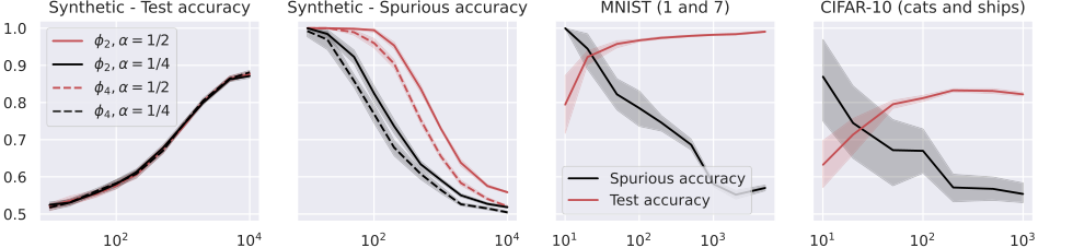 Figure 2. Test and spurious accuracies as a function of the number of training samples N, for various binary classification tasks. In the first two plots, we consider the RF model in (14) with k = 105 trained over Gaussian data with d = 1000. The labeling function is g(x) = sign(u⊤x). We repeat the experiments for α = {0.25, 0.5} and for the two activations ϕ2 = h1 + h2 and ϕ4 = h1 + h4, where hi denotes the i-th Hermite polynomial (see Appendix A.1). In the last two plots, we consider the same model with ReLU activation, trained over two MNIST and CIFAR-10 classes. The width of the noise background is 10 pixels for MNIST and 8 pixels for CIFAR-10, see Figure 1. The spurious accuracy is obtained by querying the model only with the noise background from the training set, replacing all the other pixels with 0, and taking the sign of the output. As we consider binary classification, an accuracy of 0.5 is achieved by random guessing. We plot the average over 10 independent trials and the confidence band at 1 standard deviation
- The Critical Role of Activation Functions: The experiments provided strong validation for the theoretical insight that the activation function plays a crucial role in memorization.
- For Random Features (RF) models on synthetic data (Figure 2), spurious accuracy was observed to increase with $\alpha$ (the fraction of spurious input) and when using activation functions with dominant low-order Hermite coefficients. This directly aligns with the theoretical prediction in Theorem 5.4 and Equation 17, which shows $\gamma_{RF}$ (the feature alignment constant) depends on these coefficients.
- For Neural Tangent Kernel (NTK) models on MNIST and CIFAR-10 (Figure 3), the results showed that activations with dominant high-order Hermite coefficients led to reduced memorization. This is consistent with Theorem 6.3 and Equation 26, which characterize $\gamma_{NTK}$'s dependence on the Hermite coefficients of the activation function's derivative. This demonstrates that the specific mathematical properties of the activation function, as captured by its Hermite expansion, directly dictate the model's propensity to memorize.
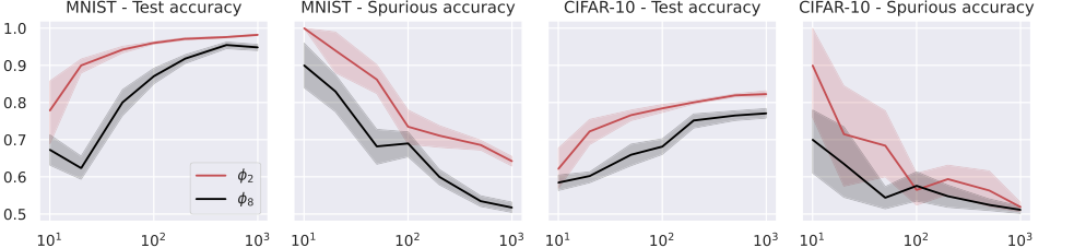 Figure 3. We consider the NTK model in (24) with k = 100, trained on MNIST (digits 1 and 7, first and second plots), and CIFAR-10 (cats and ships, third and fourth plots). We repeat the experiments for activations whose derivatives are ϕ′ 2 = h0 + h1 and ϕ′ 8 = h0 + h7, where hi denotes the i-th Hermite polynomial (see Appendix A.1). The rest of the setup is the same as that of Figure 2
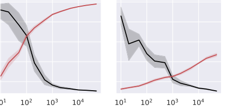 Figure 3. considers training on MNIST and CIFAR-10, and it shows that the predictions of Theorem 6.3 also hold for standard datasets: as N increases, the test accuracy im- proves and the spurious accuracy decreases; considering activations with dominant high-order Hermite coefficients reduces memorization. For additional experiments using the same setup as Figure 2 and highlighting the dependence on α, we refer the reader to Figures 6 and 7 in Appendix F
-
Dependence on the Spurious Feature Fraction ($\alpha$): Figure 7 provides compelling evidence that the spurious accuracy monotonically grows with $\alpha$ (the fraction of the input that is spurious). This was observed for both RF and NTK models on synthetic data. Crucially, the test accuracy remained largely unaffected by $\alpha$. This directly confirms the theoretical dependence of the feature alignment constants ($\gamma_{RF}$, $\gamma_{NTK}$) on $\alpha$, as established in Theorems 5.4 and 6.3. The more spurious information present, the more the model memorizes it, without necessarily improving its core task performance.
-
Broad Applicability Across Architectures: Beyond the simplified RF and NTK models, the paper extended its empirical validation to more complex deep learning architectures, including Fully Connected (FC), Convolutional Neural Networks (CNNs), and ResNets (Figures 4 and 5). These experiments showed that the observed trends—increasing test accuracy and decreasing spurious accuracy with more training samples—held true across these diverse models. This suggests that the underlying principles of memorization and its relationship to generalization, as elucidated by the feature alignment and stability framework, are not confined to linear models but are broadly applicable to modern deep learning. This provides strong support for the generality of the theoretical framework's insights, even if the precise mathematical characterization was derived for simpler models.
In essence, the experiments were architected to isolate and measure the impact of spurious features, and the consistent trends across diverse settings provide undeniable evidence that the proposed theoretical framework accurately captures the complex phenomenon of spurious feature memorization in machine learning models.
Limitations & Future Directions
While this paper provides a brilliant and precise theoretical framework for understanding how spurious features are memorized, it's important to acknowledge its current boundaries and consider how these findings can be further developed. The authors themselves offer insightful avenues for future research, which can stimulate critical thinking about the evolution of this field.
Current Limitations of the Analysis:
- Scope of Spurious Features: The primary focus of this work is on spurious features that are uncorrelated with the true learning task. While this simplifies the analysis and provides a strong foundation, many real-world spurious correlations might have some degree of correlation with the labels, making them more challenging to disentangle.
- Generalized Linear Regression Setting: The rigorous mathematical proofs for feature alignment are primarily established within the context of generalized linear regression, specifically for Random Features (RF) and Neural Tangent Kernel (NTK) models. Although empirical results suggest the insights extend to more complex deep neural networks (FC, CNN, ResNet), a full theoretical characterization for these architectures remains an open challenge.
- Specific Model Types: The exact closed-form expressions for feature alignment constants ($\gamma_{RF}$, $\gamma_{NTK}$) are derived for RF and NTK models. Extending this precise quantification to other types of models, especially those that learn features dynamically, would require significant additional theoretical work.
Future Directions & Discussion Topics:
- Spurious Features with Label Correlation: How would the memorization dynamics change if spurious features were partially correlated with the ground-truth label? This is a more realistic scenario in many applications. Could the current framework be extended to quantify the degree of "benign" versus "malicious" memorization in such cases? This would require a more nuanced definition of "spurious" that accounts for its predictive power.
- Out-of-Distribution (OOD) Spurious Features: The paper primarily examines memorization of spurious features present in the training set. What happens if a model encounters novel spurious features at test time that were not seen during training but are correlated with previously memorized spurious features? This relates directly to distribution shift robustness. Could we predict a model's vulnerability to such OOD spurious features based on its learned feature alignment?
- Integrating "Simplicity Bias": The paper mentions "simplicity bias" – the tendency of models to learn "easy" patterns first – as a related phenomenon. How can the current framework formally incorporate or explain simplicity bias? Is feature alignment a mechanism through which simplicity bias manifests, or are they distinct but interacting phenomena? Understanding this interplay could lead to more robust learning algorithms.
- Characterizing Feature Alignment for Complex Architectures: The empirical results show that the trends hold for FC, CNN, and ResNet models. A crucial next step is to theoretically characterize the feature alignment $F_\phi(z^s, z)$ for these complex, feature-learning architectures. This would involve understanding how feature maps generated by multiple fully-connected, convolutional, or attention layers influence memorization. Such a characterization would allow for direct comparison of different deep learning models' inherent susceptibility to spurious correlations.
- Designing Memorization-Resistant Models: Armed with this analytical framework, how can we design models or training strategies that are inherently less prone to memorizing spurious features? The paper highlights the role of activation functions and their Hermite coefficients. Could we engineer activation functions or architectural choices that promote higher-order feature learning, thereby reducing spurious memorization? This could involve novel regularization techniques or architectural inductive biases.
- Broader Societal Impact: While the paper explicitly states it's theoretical and doesn't delve into societal consequences, the findings have profound implications for fairness, privacy, and robustness. For instance, if a model memorizes sensitive demographic information (a spurious feature) alongside a core task, it raises privacy concerns. If it relies on spurious correlations for predictions, it can lead to biased or unfair outcomes. Future work could explore how this framework can be used to audit existing models for spurious memorization and develop interventions to mitigate these risks, thereby contributing to more ethical and trustworthy AI systems. This could involve developing metrics or tools based on feature alignment to quantify privacy leakage or fairness violations.
- Beyond Interpolation: The paper operates in the over-parameterized regime where models interpolate the training data. How do these findings translate to under-parameterized models or models that do not achieve zero training error? Do the concepts of stability and feature alignment still hold the same explanatory power in those regimes?
These discussion points highlight that this paper lays a robust theoretical groundwork, opening many exciting and challenging avenues for both theoretical and applied research in understanding and mitigating the undesirable aspects of deep learning.