Efficient Adaptation in Mixed-Motive Environments via Hierarchical Opponent Modeling and Planning
Despite the recent successes of multi-agent reinforcement learning (MARL) algorithms, efficiently adapting to co-players in mixed-motive environments remains a significant challenge.
Background & Academic Lineage
The Origin & Academic Lineage
The problem addressed in this paper, "Efficient Adaptation in Mixed-Motive Environments via Hierarchical Opponent Modeling and Planning," originates from a longstading challenge in Artificial Intelligence: enabling agents to rapidly adapt to previously unseen co-players. This capability is termed "few-shot adaptation." Historically, research in multi-agent reinforcement learning (MARL) has made significant strides in environments with predefined relationships, specifically zero-sum games (where agents are purely competitive, e.g., Vinyals et al., 2019) and common-interest environments (where agents are purely cooperative, e.g., Barrett et al., 2011).
However, the precise origin of this specific problem lies in the realization that most realistic multi-agent decision-making scenarios are not purely competitive or cooperative. Instead, they are "mixed-motive environments" (Komorita & Parks, 1995; Dafoe et al., 2020), characterized by non-deterministic relationships between agents and situations where an agent's best response can change based on others' behavior. This complexity makes decision-making and few-shot adaptation significantly more challenging than in simpler environments.
The fundamental limitation or "pain point" of previous approaches that necessitated this work stems from several issues:
1. Inapplicability of specialized techniques: Many existing MARL algorithms for few-shot adaptation rely on techniques (like minimax, Double Oracle, or IGM conditions) that are efficient for zero-sum or pure-cooperative reward structures but are not suitable for the general-sum reward structures found in mixed-motive environments.
2. Computational complexity: Methods like I-POMDP (Gmytrasiewicz & Doshi, 2005), which involve nested belief inference (i.e., an agent reasoning about what another agent thinks about its own beliefs), suffer from severe computational complexity. This makes them impractical for complex environments.
3. Information requirements and scalability issues: Algorithms such as LOLA (Foerster et al., 2018) often require knowledge of co-players' internal network parameters, which is frequently unavailable in real-world scenarios. Even when relaxed with opponent modeling, scaling problems can arise in complex sequential environments requiring long action sequences.
4. Limitations of MCTS in multi-agent settings: While Monte Carlo Tree Search (MCTS) is a powerful planning method, its application in multi-agent environments is limited because the joint action space grows exponentially with the number of agents, leading to scalability issues (Choudhury et al., 2022). Previous MCTS-based methods often struggle to estimate co-player policies efficiently.
The authors were thus compelled to develop an approach that could efficiently adapt to unseen policies in mixed-motive environments, overcoming the limitations of prior methods that were either too computationally expensive, required unavailable information, or were designed for simpler interaction dynamics. Their inspiration for a new solution came from cognitive psychology, which suggests that humans rapidly solve unseen problems using hierachical cognitive mechanisms that unify high-level goal reasoning with low-level action planning (Butz & Kutter, 2016; Eppe et al., 2022).
Intuitive Domain Terms
- Mixed-Motive Environments: Imagine a potluck dinner where everyone brings a dish. Some people want to impress everyone with their cooking (cooperative), some just want to eat as much as possible (selfish), and some might bring a simple dish but secretly hope others bring something amazing so they don't have to cook much (a mix). The "motive" of each person isn't fixed; it can be a blend of cooperation and competition, and their best strategy depends on what they think others will do.
- Few-Shot Adaptation: Think of a new employee joining a team. Instead of needing months of training to understand how each team member works, they quickly pick up on individual quirks and preferences after just a few meetings or projects. They "adapt" their own work style to fit the team after only a "few shots" (limited observations).
- Opponent Modeling: This is like a detective trying to understand a suspect's intentions. The detective observes the suspect's actions, listens to their statements, and uses this information to build a mental picture of what the suspect's goals and plans might be. The detective then uses this "model" of the opponent to predict their next move and plan their own strategy.
- Monte Carlo Tree Search (MCTS): Picture playing a complex board game like Go. Instead of trying to calculate every possible move to the end of the game (which is impossible), you quickly "imagine" playing out many random games from your current position. For each imagined game, you explore different moves, focusing more on paths that seem promising. After many such quick simulations, you pick the real move that led to the best average outcome in your mental experiments. This helps you acheive good decisions without exhaustive calculation.
- Theory of Mind (ToM): This is your ability to guess what someone else is thinking or feeling. For example, if you see someone smile, you infer they are happy. In the context of AI, it means an agent tries to understand the "mental states" (like goals, beliefs, or intentions) of other agents by observing their actions, just like humans do.
Notation Table
| Notation | Description |
|---|---|
| $N$ | Set of agents, $N = \{1, 2, \dots, n\}$ |
| $S$ | State space |
| $A_i$ | Action space for agent $i$ |
| $A$ | Joint action space, $A = A_1 \times A_2 \times \dots \times A_n$ |
| $a_{1:n}$ | Joint action taken by all agents |
| $T(s'|s, a_{1:n})$ | Transition function: probability of transitioning from state $s$ to $s'$ given joint action $a_{1:n}$ |
| $R_i$ | Reward function for agent $i$, $R_i: S \times A \to \mathbb{R}$ |
| $\gamma$ | Discount factor for future rewards |
| $T_{max}$ | Maximum length of an episode |
| $\pi_i(a_i|s)$ | Agent $i$'s policy: probability of choosing action $a_i$ at state $s$ |
| $G$ | Set of goals for all agents, $G = G_1 \times G_2 \times \dots \times G_n$ |
| $G_i$ | Set of goals for agent $i$, $G_i = \{g_{i,1}, \dots, g_{i,|G_i|}\}$ |
| $g_{i,k}$ | A specific goal for agent $i$, which is a set of states |
| $b_{i,j}(g_j)$ | Agent $i$'s belief over agent $j$'s goals, a probability distribution over $G_j$ |
| $K$ | Episode index |
| $t$ | Time step within an episode |
| $b_{i,j}^{K,t}(g_j)$ | Agent $i$'s belief about agent $j$'s goals at time $t$ in episode $K$ |
| $\pi_{\omega}(a_j|s^{K,t}, g_j)$ | Goal-conditioned policy for co-player $j$ at state $s^{K,t}$ given goal $g_j$, parameterized by $\omega$ |
| $Q_{avg}(s^{K,t}, a)$ | Average estimated action value for action $a$ at state $s^{K,t}$ |
| $\pi_{MCTS}(a|s^{K,t})$ | Policy generated by MCTS for action $a$ at state $s^{K,t}$ |
| $\beta$ | Rationality coefficient for Boltzmann rationality model |
| $N_s$ | Number of MCTS rounds |
| $N_l$ | Number of search iterations for each MCTS round |
| $c$ | Exploration coefficient for MCTS |
| $\theta$ | Parameters of the policy and value network for MCTS |
| $\omega$ | Parameters of the goal-conditioned policy network |
Problem Definition & Constraints
Core Problem Formulation & The Dilemma
The central challenge addressed by this paper is the efficient few-shot adaptation to unseen co-players in mixed-motive multi-agent environments. This is a critical problem in Artificial Intelligence, as most real-world interactions involve a blend of cooperation and competition, rather than purely competitive (zero-sum) or purely cooperative (common-interest) dynamics.
Starting Point (Input/Current State):
Current multi-agent reinforcement learning (MARL) algorithms, despite successes in zero-sum and common-interest games, largely struggle in mixed-motive settings. These environments are characterized by non-deterministic relationships between agents and general-sum reward structures, making decision-making inherently more complex. Previous approaches to opponent modeling often face two significant hurdles:
1. Inefficient Reasoning: Existing methods, such as I-POMDP and its approximations, suffer from "serious computational complexity problems" due to nested belief inference, rendering them impractical in complex environments.
2. Ineffective Utilization of Inferred Information: Algorithms like LOLA, while considering opponent learning, often require knowledge of co-players' internal network parameters, which is frequently unavailable in realistic scenarios. Furthermore, many existing algorithms rely on hand-crafted intrinsic rewards or assume access to co-players' private rewards, making them susceptible to exploitation by self-interested agents or less effective when such information is hidden. Monte Carlo Tree Search (MCTS), a powerful planning tool, also faces limitations in multi-agent settings where the joint action space expands rapidly with the number of agents.
Desired Endpoint (Output/Goal State):
The paper aims to develop an algorithm that enables a focal agent to achieve "few-shot adaptation to unseen policies" in mixed-motive environments. This means the agent should be able to:
1. Rapidly Adapt: Quickly recognize and respond appropriately to new, previously unseen co-players within a limited number of episodes.
2. Efficiently Reason and Utilize Information: Infer co-players' goals and learn their goal-conditioned policies efficiently, and then leverage this inferred information to compute optimal responses without incurring prohibitive computational costs.
3. Perform Robustly: Make autonomous decisions that yield high rewards in mixed-motive scenarios, even when co-players' goals are private and potentially volatile.
The Exact Missing Link or Mathematical Gap:
The precise gap this paper attempts to bridge is the lack of a scalable and efficient framework for hierarchical opponent modeling and planning under uncertainty in mixed-motive environments. Specifically, it addresses how to:
* Accurately infer co-players' latent goals and goal-conditioned policies from their observed actions, rather than relying on direct access to their internal parameters or hand-crafted rewards.
* Integrate this inferred opponent model into a planning mechanism (MCTS) in a way that remains computationally tractable, avoiding the "nested belief inference" issues of prior methods.
* Handle the inherent uncertainty about co-players' goals during planning without introducing significant bias or degrading performance. The paper proposes a hierarchical structure with "intra-OM" and "inter-OM" modules to update beliefs about co-players' goals both within and across episodes, and then uses these beliefs to guide an MCTS planner that samples multiple goal combinations to compute the best response.
The Painful Trade-off or Dilemma:
The core dilemma that has trapped previous researchers is the trade-off between the accuracy and generalizability of opponent modeling versus its computational efficiency and scalability.
* Accuracy vs. Efficiency: Achieving highly accurate models of diverse co-players, especially in complex mixed-motive settings where goals are private and dynamic, typically demands extensive computation (e.g., nested belief inference in I-POMDP) or detailed knowledge of opponent internals (e.g., LOLA). This often makes such methods too slow or resource-intensive for rapid, few-shot adaptation in real-time or complex sequential environments.
* Generalizability vs. Specificity: Algorithms designed for specific game types (zero-sum or pure-cooperative) often leverage reward-structure-specific techniques (e.g., minimax) that do not generalize to the non-deterministic, general-sum nature of mixed-motive interactions. Developing a method that works across the spectrum of mixed motives without sacrificing performance in any specific area is a significant challenge. The paper aims for a "practical and effective framework" that can handle both competition and cooperation.
Constraints & Failure Modes
The problem of efficient few-shot adaptation in mixed-motive environments is "insanely difficult" due to several harsh, realistic constraints:
Physical/Environmental Constraints:
* Mixed-Motive Dynamics: The fundamental constraint is the environment itself. Relationships between agents are "non-deterministic," and reward structures are "general-sum," meaning agents' interests are neither perfectly aligned nor perfectly opposed. This makes predicting optimal responses highly context-dependent and dynamic.
* Unseen Co-players and Policies: The requirement for "few-shot adaptation to unseen agents" means the algorithm cannot rely on pre-training with specific opponent types. Agents must adapt to novel behaviors on the fly.
* Limited Interaction History: "Few-shot adaptation" implies that the agent has only a "limited number of episodes" to learn about new co-players. This severely restricts the amount of data available for opponent modeling and adaptation.
* Private Goals and No Communication: Agents have "no access to each other's parameters, and communication is not allowed." Furthermore, co-players' goals are "private and volatile," meaning they can change within an episode. This lack of direct information necessitates inferring intentions solely from observed actions.
Computational Constraints:
* Computational Complexity of Opponent Modeling: Previous methods like I-POMDP are plagued by "serious computational complexity problems" due to "nested belief inference," making them impractical for complex environments. The challenge is to model opponents accurately without exponential growth in computation.
* Scaling with Number of Agents: In multi-agent environments, the "joint action space grows rapidly with the number of agents." This makes planning with traditional MCTS computationally prohibitive for many agents. The paper explicitly addresses this by planning only for the focal agent's actions, given estimated co-player policies.
* Real-time Latency Requirements (Implicit): The need for "rapid adaptation" and "efficient reasoning" implies that decision-making must occur within practical time limits, especially in sequential decision-making scenarios that might involve long action sequences.
Data-Driven Constraints:
* Data Sparsity for Belief Updates: When "past trajectories are not long enough for updates," the intra-episode opponent modeling (intra-OM) can suffer from "inaccuracy of the prior." This highlights the difficulty of forming accurate beliefs about co-players' goals from minimal data.
* Uncertainty in Co-player Models: Even with opponent modeling, the estimated co-player policies "contain uncertainty over co-players' goals." This uncertainty must be effectively managed during the planning phase to avoid introducing "large bias to the simulation and degrade planning performance." Naively incorporating this uncertainty can lead to suboptimal actions.
Why This Approach
The Inevitability of the Choice
The adoption of Hierarchical Opponent modeling and Planning (HOP) was not merely a design choice but an inevitable consequence of the inherent challenges posed by mixed-motive environments. Traditional state-of-the-art (SOTA) multi-agent reinforcement learning (MARL) algorithms, such as those relying on minimax, Double Oracle, or IGM conditions, were found to be fundamentally insufficient. These methods are tailored for specific reward structures found in zero-sum or purely cooperative games, making them "not applicable in mixed-motive environments" where agent relationships are non-deterministic and rewards are general-sum. The authors explicitly state that the "non-deterministic relationships between agents and the general-sum reward structure make decision-making and few-shot adaptation more challenging in mixed-motive environments compared with zero-sum and pure-cooperative environments."
The realization that existing methods were inadequate led the authors to seek inspiration from cognitive psychology. They identified that humans' ability to rapidly solve previously unseen problems hinges on "hierarchical cognitive mechanisms" that seamlessly integrate high-level goal reasoning with low-level action planning. This insight was the exact moment the authors recognized the need for a fundamentally different, hierarchically structured approach. HOP directly mirrors this cognitive architecture, proposing an opponent modeling module for inferring co-players' goals and learning goal-conditioned policies, coupled with a planning module that uses Monte Carlo Tree Search (MCTS) to determine the best response. This hierarchical decomposition was the only viable path to address the dual challenges of efficient reasoning and effective utilization of inferred information in complex, mixed-motive settings.
Comparative Superiority
HOP demonstrates qualitative superiority over previous gold standards through several structural advantages that go beyond simple performance metrics:
- Hierarchical Decomposition: Unlike flat MARL approaches, HOP's two-module structure (opponent modeling and planning) allows for a more sophisticated and interpretable understanding of co-player behavior. The opponent modeling module infers high-level goals and learns goal-conditioned policies, providing a richer representation than direct end-to-end models. This mirrors human cognitive processes, enabling more robust adaptation.
- Efficient Belief Update Mechanism: HOP significantly improves efficiency by updating beliefs about co-players' goals both across and within episodes. The intra-opponent modeling (intra-OM) module allows for rapid adjustments to co-players' immediate goals within a single episode, crucial for dynamic environments. The inter-opponent modeling (inter-OM) module leverages historical episodes to establish a precise prior belief, accelerating convergence to true beliefs. This dual-layer update mechanism provides a structural advantage over methods that might only update beliefs within an episode or lack a robust historical context, which often leads to inaccurate opponent modeling during short interactions.
- Avoidance of Nested Belief Inference Complexity: Previous opponent modeling and planning frameworks, such as I-POMDP, suffer from "serious computational complexity problems" due to "nested belief inference" (e.g., an agent reasoning about what another agent thinks it thinks). HOP circumvents this by explicitly using beliefs over co-players' goals and policies to learn a neural network model, which then guides an MCTS planner. This design choice allows HOP to "perform sequential decision-making more efficiently" without the computational bottleneck of deep recursive reasoning.
- Scalable MCTS Integration: While MCTS is powerful, its direct application in multi-agent environments is limited by the rapid growth of the joint action space. HOP overcomes this by "estimating the policies of co-players and planning only for the focal agent's actions." This strategic decoupling allows MCTS to be applied effectively and scalably, avoiding the computational explosion associated with planning over all agents' joint actions.
- Reduced Uncertainty in Planning: The opponent modeling module provides goal-conditioned policies to the planning module. This inferred information guides MCTS, preventing the "large bias" and "degraded planning performance" that would result from naively incorporating uncertainty about co-players' goals directly into the environment model for planning. This structural integration ensures that planning is informed and precise, even under uncertainty.
Alignment with Constraints
HOP's design perfectly aligns with the harsh requirements of few-shot adaptation in mixed-motive environments:
- Few-Shot Adaptation to Unseen Policies: The core objective of HOP is few-shot adaptation. The hierarchical structure, particularly the efficient intra-OM and inter-OM belief update mechanisms, is specifically engineered for this. Intra-OM allows for quick responses to in-episode behavior changes, while inter-OM provides accurate priors from past episodes, enabling rapid adaptation to novel co-player strategies within a limited number of interactions. This "marriage" between the problem's need for rapid learning and the solution's dynamic belief updates is fundamental.
- Mixed-Motive Environments: HOP is purpose-built for mixed-motive scenarios, where relationships are non-deterministic and rewards are general-sum. Its ability to infer co-players' goals (which can be competitive, cooperative, or mixed) and plan the focal agent's best response, even when co-players' goals are private and volatile, directly addresses the central challenge of these environments.
- No Access to Co-player Parameters or Rewards: A critical constraint in realistic multi-agent settings is the lack of direct access to other agents' internal parameters or reward functions. HOP's opponent modeling module infers co-players' goals and learns their goal-conditioned policies solely by observing their "action sequences." This inference-based approach bypasses the need for explicit knowledge of co-players' internals, making it applicable in real-world, black-box scenarios.
- No Communication: The problem definition implies a lack of explicit communication between agents. HOP's goal inference and policy learning are entirely based on observed trajectories and actions, without relying on any form of direct communication, thus adhering to this implicit constraint.
Rejection of Alternatives
The paper provides clear reasoning for rejecting several popular approaches:
- Traditional MARL Algorithms (e.g., Minimax, Double Oracle, IGM condition): These methods are explicitly rejected because they are "not applicable in mixed-motive environments." Their underlying assumptions and techniques are optimized for zero-sum or pure-cooperative reward structures, which fail to capture the non-deterministic relationships and general-sum rewards characteristic of mixed-motive games.
- LOLA (Learning with Opponent-Learning Awareness): While an advanced MARL algorithm, LOLA is deemed unsuitable for general mixed-motive environments because it "requires knowledge of co-players' network parameters, which may not be feasible in many scenarios." HOP's inference-based opponent modeling avoids this restrictive requirement. Furthermore, LOLA can suffer from "scaling problems... in complex sequential environments that require long action sequences for rewards," a limitation HOP addresses through its guided MCTS planning.
- I-POMDP (Interactive Partially Observable Markov Decision Processes): This framework, though relevant to opponent modeling, is rejected due to its "serious computational complexity problems" stemming from "nested belief inference." The computational burden makes it "impractical in complex environments." HOP's design specifically avoids this nested inference to achieve greater efficiency.
- Naive MCTS in Multi-Agent Environments: The paper acknowledges that MCTS alone is "limited in multi-agent environments, where the joint action space grows rapidly with the number of agents." A direct application would be computationally intractable. HOP's solution is to estimate co-player policies and plan only for the focal agent's actions, effectively sidestepping this scalability issue.
- Ablated HOP Versions (w/o inter-OM, w/o intra-OM, direct-OM): The ablation study provides empirical evidence for rejecting simpler or incomplete versions of HOP:
- W/o inter-OM: This version struggles against agents with fixed goals (e.g., cooperators, defectors) because it lacks accurate goal priors at the start of an episode, missing early opportunities for optimal play. This highlights the necessity of leveraging historical episodes.
- W/o intra-OM: This version performs poorly against agents with dynamic behaviors (e.g., LOLA, PS-A3C, random) because it cannot adapt to in-episode changes in co-players' goals, relying only on past episodes. This underscores the importance of real-time, within-episode belief updates.
- Direct-OM: This approach, which removes the hierarchical opponent modeling module and uses neural networks to model co-players directly without goal conditioning, is at an "overall disadvantage." It struggles to obtain significant updates during short interactions, leading to "inaccurate opponent modeling during the adaptation phase." The end-to-end nature also introduces "a higher degree of uncertainty compared to the goal-conditioned policy," reducing planning precision. This clearly validates the superiority of HOP's goal-conditioned, hierarchical opponent modeling.
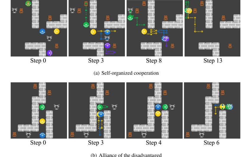 Figure 6. Screenshots for the emergence of (a) self-organized cooperation and (b) alliance of the disadvantaged. Each panel shows agents’ locations at the current step and the trajectories between the current step and the previously stated step
Mathematical & Logical Mechanism
The Master Equation
The Hierarchical Opponent modeling and Planning (HOP) algorithm is powered by several interconnected mathematical mechanisms that enable its adaptive capabilities. At its core, HOP relies on Bayesian inference for opponent goal modeling, a negative log-likelihood objective for learning goal-conditioned opponent policies, and a combined policy and value loss for training the focal agent's decision-making networks, guided by Monte Carlo Tree Search (MCTS).
The absolute core equations that define HOP's mathematical engine are:
-
Intra-Episode Opponent Goal Belief Update (Intra-OM): This equation updates the focal agent's belief about a co-player's goal within a single episode, incorporating real-time observations.
$$b_{ij}^{K,t+1}(g_j) = \frac{1}{Z_1} b_{ij}^{K,t}(g_j) \frac{\Pr(a_j^{K,t}|s^{K,t}, g_j) \Pr(s^{K,t+1}|s^{K,t}, a_j^{K,t}, g_j)}{\Pr(s^{K,t+1}|s^{K,t}, a_j^{K,t})}$$ -
Inter-Episode Opponent Goal Belief Update (Inter-OM): This equation updates the prior belief about a co-player's goal at the start of a new episode, leveraging information from past episodes.
$$b_{ij}^{K,0}(g_j) = \frac{1}{Z_2} [\alpha b_{ij}^{K-1,0}(g_j) + (1-\alpha)\mathbf{1}(g_j = g_j^{K-1})]$$ -
Goal-Conditioned Opponent Policy Network Loss: This objective function trains the neural network that predicts co-players' actions given their inferred goals and the current state.
$$\mathcal{L}(\omega) = \mathbb{E}[-\log(\pi_\omega(a_j^{K,t}|s^{K,t}, g_j^{K,t}))]$$ -
Focal Agent's Policy and Value Network Loss: This combined loss function trains the focal agent's main policy and value networks, using MCTS as a supervisor.
$$\mathcal{L}(\theta) = \mathcal{L}_p(\pi_{\text{MCTS}}, \pi_\theta) + \mathcal{L}_v(r_i, v_\theta)$$
where
$$\mathcal{L}_p(\pi_1, \pi_2) = \mathbb{E}[-\sum_{a \in \mathcal{A}_i} \pi_1(a|s^{K,t}) \log(\pi_2(a|s^{K,t}))]$$
$$\mathcal{L}_v(r_i, v) = \mathbb{E}[(v(s^{K,t}) - \sum_{l=t}^{T_{\text{max}}} \gamma^{l-t} r_i^{K,l})^2]$$
Term-by-Term Autopsy
Let's dissect each of these equations to understand the role of every component.
Intra-Episode Opponent Goal Belief Update (Equation 1)
$$b_{ij}^{K,t+1}(g_j) = \frac{1}{Z_1} b_{ij}^{K,t}(g_j) \frac{\Pr(a_j^{K,t}|s^{K,t}, g_j) \Pr(s^{K,t+1}|s^{K,t}, a_j^{K,t}, g_j)}{\Pr(s^{K,t+1}|s^{K,t}, a_j^{K,t})}$$
- $b_{ij}^{K,t+1}(g_j)$:
- Mathematical Definition: The posterior probability distribution representing agent $i$'s belief about opponent $j$'s goal $g_j$ at time $t+1$ within episode $K$.
- Physical/Logical Role: This is the updated belief. It tells the focal agent, "Given everything I've seen up to now in this episode, how likely is it that opponent $j$ has goal $g_j$?" It's crucial for real-time adaptation to co-players' changing behaviors.
- $Z_1$:
- Mathematical Definition: A normalization factor.
- Physical/Logical Role: Ensures that the sum of probabilities for all possible goals $g_j$ for opponent $j$ equals 1, maintaining a valid probability distribution.
- Why division: It's a fundamental part of Bayes' theorem to scale the numerator (prior times likelihood) into a proper probability.
- $b_{ij}^{K,t}(g_j)$:
- Mathematical Definition: The prior probability distribution representing agent $i$'s belief about opponent $j$'s goal $g_j$ at time $t$ within episode $K$.
- Physical/Logical Role: This is the belief before observing the latest action and state transition. It serves as the starting point for the current Bayesian update step.
- $\Pr(a_j^{K,t}|s^{K,t}, g_j)$:
- Mathematical Definition: The probability of opponent $j$ taking action $a_j^{K,t}$ given the current state $s^{K,t}$ and a hypothesized goal $g_j$. This is provided by the goal-conditioned policy network $\pi_\omega$.
- Physical/Logical Role: This term acts as the "likelihood of the action." It quantifies how well a particular hypothesized goal $g_j$ explains the observed action $a_j^{K,t}$. If an opponent takes an action that is very likely under goal $g_A$ but unlikely under goal $g_B$, this term will boost the belief in $g_A$.
- $\Pr(s^{K,t+1}|s^{K,t}, a_j^{K,t}, g_j)$:
- Mathematical Definition: The probability of transitioning to state $s^{K,t+1}$ given the previous state $s^{K,t}$, opponent $j$'s action $a_j^{K,t}$, and a hypothesized goal $g_j$. The paper mentions a Markov assumption where this might simplify to $\Pr(s^{K,t+1}|s^{K,t}, a_j^{K,t})$, implying independence from $g_j$ given the action. However, the equation includes $g_j$, suggesting a potential dependence or a more general formulation.
- Physical/Logical Role: This term acts as the "likelihood of the state transition." It further refines the belief by considering if the observed state change is consistent with the hypothesized goal and action.
- $\Pr(s^{K,t+1}|s^{K,t}, a_j^{K,t})$:
- Mathematical Definition: The probability of transitioning to state $s^{K,t+1}$ given the previous state $s^{K,t}$ and opponent $j$'s action $a_j^{K,t}$.
- Physical/Logical Role: This is a normalization term for the state transition likelihood, ensuring the overall likelihood is properly scaled.
- Why multiplication: Bayesian updates combine prior beliefs with likelihoods through multiplication, reflecting how new evidence scales the existing belief.
Inter-Episode Opponent Goal Belief Update (Equation 2)
$$b_{ij}^{K,0}(g_j) = \frac{1}{Z_2} [\alpha b_{ij}^{K-1,0}(g_j) + (1-\alpha)\mathbf{1}(g_j = g_j^{K-1})]$$
- $b_{ij}^{K,0}(g_j)$:
- Mathematical Definition: The prior probability distribution representing agent $i$'s belief about opponent $j$'s goal $g_j$ at the start of episode $K$.
- Physical/Logical Role: This is the initial guess for opponent $j$'s goal in a new episode. It's informed by past experiences, providing a "memory" of opponent behavior.
- $Z_2$:
- Mathematical Definition: A normalization factor.
- Physical/Logical Role: Ensures the sum of probabilities for all possible goals $g_j$ equals 1.
- Why division: Standard normalization for probability distributions.
- $\alpha$:
- Mathematical Definition: A horizon weight, $\alpha \in [0, 1]$.
- Physical/Logical Role: This coefficient controls the influence of historical beliefs versus the most recently observed goal. A higher $\alpha$ means older beliefs are more important, leading to slower adaptation. A lower $\alpha$ (closer to 0) means the agent prioritizes the goal observed in the immediately preceding episode, enabling faster adaptation to dynamic opponents.
- Why multiplication: It scales the contribution of the previous episode's prior belief.
- $b_{ij}^{K-1,0}(g_j)$:
- Mathematical Definition: The prior probability distribution over opponent $j$'s goals $g_j$ for agent $i$ at the start of the previous episode $K-1$.
- Physical/Logical Role: Represents the accumulated historical knowledge about opponent $j$'s goals from all episodes prior to the current one.
- $(1-\alpha)$:
- Mathematical Definition: The complementary weight to $\alpha$.
- Physical/Logical Role: Scales the contribution of the observed goal from the previous episode.
- Why multiplication: It scales the contribution of the most recent goal observation.
- $\mathbf{1}(g_j = g_j^{K-1})$:
- Mathematical Definition: An indicator function that returns 1 if opponent $j$'s goal in the previous episode $K-1$ was $g_j$, and 0 otherwise.
- Physical/Logical Role: This term directly incorporates the actual goal that was inferred for opponent $j$ in the last episode. It's a strong signal for updating the prior for the new episode.
- Why addition: The two weighted terms are added to combine the long-term historical belief with the short-term, most recent observation to form the new prior.
Goal-Conditioned Opponent Policy Network Loss (Equation 3)
$$\mathcal{L}(\omega) = \mathbb{E}[-\log(\pi_\omega(a_j^{K,t}|s^{K,t}, g_j^{K,t}))]$$
- $\mathcal{L}(\omega)$:
- Mathematical Definition: The loss function for the goal-conditioned policy network, parameterized by $\omega$.
- Physical/Logical Role: This is the objective that the opponent modeling module minimizes to learn accurate goal-conditioned policies for co-players. A lower loss means the network is better at predicting opponent actions given their goals.
- $\mathbb{E}[\cdot]$:
- Mathematical Definition: The expectation operator, typically approximated by averaging over a batch of data samples from the replay buffer.
- Physical/Logical Role: Provides a stable estimate of the loss by averaging over multiple observations, reducing the impact of noise from individual data points during training.
- $-\log(\pi_\omega(a_j^{K,t}|s^{K,t}, g_j^{K,t}))$:
- Mathematical Definition: The negative logarithm of the probability assigned by the policy network $\pi_\omega$ to the observed action $a_j^{K,t}$, given the state $s^{K,t}$ and the inferred goal $g_j^{K,t}$.
- Physical/Logical Role: This is the standard negative log-likelihood loss used in supervised learning for classification or policy learning. Minimizing this term maximizes the probability that the network assigns to the correct (observed) action, effectively teaching the network to mimic opponent behavior under specific goals.
- Why negative log: The logarithm transforms products of probabilities into sums, which are easier to optimize. The negative sign converts the objective from maximizing likelihood to minimizing loss, which is standard for gradient-based optimization.
Focal Agent's Policy and Value Network Loss (Equation 6)
$$\mathcal{L}(\theta) = \mathcal{L}_p(\pi_{\text{MCTS}}, \pi_\theta) + \mathcal{L}_v(r_i, v_\theta)$$
$$\mathcal{L}_p(\pi_1, \pi_2) = \mathbb{E}[-\sum_{a \in \mathcal{A}_i} \pi_1(a|s^{K,t}) \log(\pi_2(a|s^{K,t}))]$$
$$\mathcal{L}_v(r_i, v) = \mathbb{E}[(v(s^{K,t}) - \sum_{l=t}^{T_{\text{max}}} \gamma^{l-t} r_i^{K,l})^2]$$
- $\mathcal{L}(\theta)$:
- Mathematical Definition: The total loss function for the focal agent's policy and value networks, parameterized by $\theta$.
- Physical/Logical Role: This is the primary objective function that the focal agent minimizes to learn its optimal policy and an accurate value function. It combines two critical aspects of reinforcement learning: learning to act well and learning to predict future rewards.
- Why addition: Policy and value learning are often combined into a single objective in actor-critic or AlphaZero-like architectures, as they are complementary tasks that benefit from shared representations and joint optimization.
- $\mathcal{L}_p(\pi_{\text{MCTS}}, \pi_\theta)$:
- Mathematical Definition: The policy loss term, specifically a cross-entropy loss between the MCTS-derived policy $\pi_{\text{MCTS}}$ (target policy $\pi_1$) and the learned policy $\pi_\theta$ (predicted policy $\pi_2$).
- Physical/Logical Role: This term acts as a "policy distillation" mechanism. MCTS, through its look-ahead search, generates a superior policy. This loss encourages the focal agent's learned policy $\pi_\theta$ to imitate and internalize the MCTS-generated policy, effectively transferring the "wisdom" of planning into the neural network.
- $\mathbb{E}[-\sum_{a \in \mathcal{A}_i} \pi_1(a|s^{K,t}) \log(\pi_2(a|s^{K,t}))]$:
- Mathematical Definition: The cross-entropy between two probability distributions $\pi_1$ and $\pi_2$.
- Physical/Logical Role: Measures how different the learned policy $\pi_2$ is from the MCTS target policy $\pi_1$. Minimizing cross-entropy makes $\pi_2$ match $\pi_1$.
- Why summation: Sums the negative log-probabilities over all possible actions in the focal agent's action space $\mathcal{A}_i$, weighted by the target policy's probabilities.
- $\mathcal{L}_v(r_i, v_\theta)$:
- Mathematical Definition: The value loss term, specifically a mean squared error (MSE) between the predicted value $v(s^{K,t})$ from the value network and the true discounted return $\sum_{l=t}^{T_{\text{max}}} \gamma^{l-t} r_i^{K,l}$.
- Physical/Logical Role: This term trains the value network $v_\theta$ to accurately predict the expected cumulative future rewards from any given state. A precise value function is crucial for guiding MCTS and for evaluating the quality of states.
- $\mathbb{E}[(v(s^{K,t}) - \sum_{l=t}^{T_{\text{max}}} \gamma^{l-t} r_i^{K,l})^2]$:
- Mathematical Definition: The squared difference between the predicted value and the actual discounted return.
- Physical/Logical Role: This is a standard regression loss. It penalizes the value network for inaccurate predictions, with larger errors receiving quadratically higher penalties.
- Why squared difference: Common for regression tasks, it provides a smooth, differentiable loss landscape for gradient-based optimization.
- $v(s^{K,t})$:
- Mathematical Definition: The value predicted by the focal agent's value network for state $s^{K,t}$.
- Physical/Logical Role: The model's current estimate of the total future discounted reward obtainable from state $s^{K,t}$.
- $\sum_{l=t}^{T_{\text{max}}} \gamma^{l-t} r_i^{K,l}$:
- Mathematical Definition: The true discounted return (cumulative reward) received by agent $i$ from time step $t$ until the end of the episode $T_{\text{max}}$.
- Physical/Logical Role: This is the "ground truth" for the value network. It represents the actual sum of future rewards, discounted by their temporal distance.
- Why summation: Accumulates rewards over the entire future trajectory.
- $\gamma$:
- Mathematical Definition: The discount factor, $\gamma \in [0, 1]$.
- Physical/Logical Role: Determines the present value of future rewards. A $\gamma$ close to 0 makes the agent myopic (cares only about immediate rewards), while a $\gamma$ close to 1 makes it far-sighted (considers long-term rewards heavily).
- Why exponentiation: Standard in reinforcement learning to exponentially decrease the importance of rewards further in the future.
Step-by-Step Flow
Imagine a single abstract data point, say, an observation of the environment state and co-players' actions, entering the HOP system. Here's how it moves through the mathematical engine:
-
Episode Start: Setting the Stage with History:
- When a new episode $K$ begins, the focal agent $i$ doesn't start from scratch regarding its beliefs about co-players. It first consults its "memory" of past interactions.
- The Inter-OM belief update (Equation 2) is triggered. This equation takes the prior belief from the previous episode, $b_{ij}^{K-1,0}(g_j)$, and combines it with the actual goal $g_j^{K-1}$ that was inferred for opponent $j$ in that last episode. The horizon weight $\alpha$ acts like a dial, blending how much to trust the long-term history versus the very recent past. This produces an initial belief $b_{ij}^{K,0}(g_j)$ for the current episode, giving the agent a head start.
-
Real-time Interaction: Observing and Inferring Opponent Goals:
- As the episode unfolds, at each time step $t$, the agent observes the current state $s^{K,t}$ and the actions $a_j^{K,t}$ taken by its co-players.
- This new observation immediately feeds into the Intra-OM belief update (Equation 1). The agent takes its current belief $b_{ij}^{K,t}(g_j)$ (which was $b_{ij}^{K,0}(g_j)$ at $t=0$) and updates it. It asks: "How likely is it that opponent $j$ would have taken action $a_j^{K,t}$ and caused state $s^{K,t+1}$ if their goal was $g_j$?"
- To answer this, it uses the goal-conditioned policy network $\pi_\omega$ to get $\Pr(a_j^{K,t}|s^{K,t}, g_j)$ for each possible goal $g_j$. This likelihood is then multiplied by the current belief, and the result is normalized by $Z_1$. This process continuously refines $b_{ij}^{K,t+1}(g_j)$, making the belief about opponent goals more accurate as more actions are observed within the episode.
-
Learning Opponent Behavior: Training the Goal-Conditioned Policy:
- Throughout this process, the inferred goals $g_j^{K,t}$ (the most likely goals) along with the observed states $s^{K,t}$ and actions $a_j^{K,t}$ are collected and stored in a trajectory buffer.
- Periodically, this collected data is used to train the goal-conditioned policy network $\pi_\omega$. The Goal-Conditioned Policy Network Loss (Equation 3) is minimized. This is like a teacher showing the network examples: "When the opponent was in state $s$ with goal $g$, they took action $a$." The network learns to predict $a$ given $s$ and $g$, improving its ability to model co-players' behavior.
-
Focal Agent's Decision-Making: Planning for the Best Response:
- Now, it's the focal agent's turn to act. It needs to choose its own action $a_i^{K,t}$.
- The agent initiates Monte Carlo Tree Search (MCTS). MCTS doesn't just consider the current state; it simulates many possible futures.
- Crucially, MCTS doesn't know co-players' goals for sure. So, in each of its $N_s$ simulation rounds, it samples a combination of co-players' goals $g_{-i}$ from the current belief $b_{ij}^{K,t}(g_j)$ (from step 2).
- For each sampled goal combination, MCTS simulates trajectories. When it needs to know what a co-player $j$ would do, it uses the learned goal-conditioned policy $\pi_\omega(\cdot|s, g_j)$ (from step 3) with the sampled goal $g_j$. The focal agent explores its own actions.
- After $N_s$ rounds, MCTS calculates an average action value $Q_{\text{avg}}(s^{K,t}, a)$ (Equation 4) for each of the focal agent's possible actions, considering the uncertainty over co-players' goals.
- Finally, the focal agent selects its action $a_i^{K,t}$ using a Boltzmann rationality model (Equation 5), which favors actions with higher $Q_{\text{avg}}$ values, balancing exploration and exploitation.
-
Learning to Be Better: Training the Focal Agent's Networks:
- The MCTS process itself provides valuable information: a "better" policy $\pi_{\text{MCTS}}$ (derived from the search) and an improved estimate of the state's value.
- This information, along with the actual rewards $r_i^{K,l}$ received, is used to train the focal agent's main policy and value networks, parameterized by $\theta$.
- The Focal Agent's Policy and Value Network Loss (Equation 6) is minimized. This loss has two parts:
- A policy loss $\mathcal{L}_p$ that makes the learned policy $\pi_\theta$ mimic the MCTS-generated policy $\pi_{\text{MCTS}}$. This is like the MCTS "teacher" showing the network the optimal moves.
- A value loss $\mathcal{L}_v$ that makes the value network $v_\theta$ accurately predict the true discounted returns $\sum_{l=t}^{T_{\text{max}}} \gamma^{l-t} r_i^{K,l}$ observed during the episode. This teaches the network to correctly assess how good a state is.
- Through this combined loss, the focal agent's neural networks learn to make better decisions and evaluate states more accurately, becoming more proficient over time.
This entire cycle repeats, with each step feeding into and improving the others, creating a dynamic and adaptive learning system.
Optimization Dynamics
The HOP mechanism learns, updates, and converges through a continuous, iterative process that refines its understanding of opponents and its own decision-making capabilities. This learning is driven by gradient descent on various loss functions and the inherent self-improvement of MCTS.
-
Belief System Refinement:
- Intra-episode Beliefs (Equation 1): The intra-OM module continuously updates beliefs about co-players' goals using Bayesian inference. Each new observation (opponent action and state transition) provides evidence that either strengthens or weakens the probability of a particular goal. Over time, as more data is collected within an episode, the posterior distribution $b_{ij}^{K,t+1}(g_j)$ tends to converge towards the true underlying goal of the opponent, assuming their behavior is consistent with one of the learned goal-conditioned policies. This is a classic Bayesian update, where the uncertainty (entropy) in the belief distribution decreases with accumulating evidence.
- Inter-episode Priors (Equation 2): The inter-OM module updates the prior belief for new episodes. The horizon weight $\alpha$ is a critical hyperparameter here. If $\alpha$ is high, the system relies heavily on long-term historical averages, leading to slow but stable convergence of the prior belief. If $\alpha$ is low, the system adapts quickly to recent opponent behaviors, potentially leading to faster adaptation but also more instability if opponent goals are highly volatile. This mechanism allows the system to track and adapt to shifts in opponent strategies across multiple episodes.
-
Opponent Policy Learning:
- The goal-conditioned policy network $\pi_\omega$ (used to predict opponent actions) is trained by minimizing the negative log-likelihood loss (Equation 3) using stochastic gradient descent (SGD) or its variants. The loss landscape for this network is shaped by the accuracy of its predictions against observed opponent actions. As more diverse and accurate data (state, inferred goal, actual action) is collected and fed into the replay buffer, the gradients guide the network parameters $\omega$ to minimize this loss. This process iteratively improves the network's ability to accurately model opponent behavior, making the opponent modeling module more reliable.
-
Focal Agent's Policy and Value Learning:
- The focal agent's policy $\pi_\theta$ and value function $v_\theta$ are learned through a supervised process where MCTS acts as a powerful "teacher." The overall loss $\mathcal{L}(\theta)$ (Equation 6) is minimized using gradient descent.
- Policy Improvement: MCTS, by performing extensive simulations and look-ahead searches, generates a "stronger" policy $\pi_{\text{MCTS}}$ than the current learned policy $\pi_\theta$. The policy loss term $\mathcal{L}_p$ then drives $\pi_\theta$ to mimic $\pi_{\text{MCTS}}$. This means the gradients from $\mathcal{L}_p$ pull the parameters $\theta$ in a direction that makes the learned policy more closely resemble the MCTS-derived optimal actions. This iterative supervision allows $\pi_\theta$ to converge towards a near-optimal policy without needing to directly explore the environment.
- Value Function Accuracy: The value loss term $\mathcal{L}_v$ trains $v_\theta$ to predict the true discounted returns observed during the MCTS simulations and actual gameplay. The gradients from $\mathcal{L}_v$ guide $\theta$ to reduce the mean squared error between predicted and actual returns. As $v_\theta$ becomes more accurate, it provides better estimates for MCTS, allowing the search to be more efficient and effective. This creates a positive feedback loop: better value estimates lead to better MCTS, which leads to better training targets for $v_\theta$.
- Loss Landscape: The combined loss $\mathcal{L}(\theta)$ creates a complex loss landscape. However, the MCTS supervision provides a strong, albeit potentially noisy, signal that guides the neural network parameters $\theta$ towards regions of higher expected return. The iterative nature of MCTS (repeated simulations) and neural network training (gradient updates) allows the system to converge to a robust policy and value function.
-
MCTS Exploration-Exploitation:
- The MCTS algorithm itself balances exploration and exploitation using mechanisms like pUCT (Polynomial Upper Confidence Trees). The exploration coefficient $c$ in the MCTS score function (mentioned in Appendix E.1) controls this balance. A higher $c$ encourages MCTS to explore less-visited actions, potentially discovering better strategies. A lower $c$ makes MCTS exploit known good actions more, leading to faster convergence to local optima. This dynamic ensures that MCTS continues to find improved policies to supervise the neural network.
In summary, HOP's optimization dynamics are characterized by a hierarchical and iterative learning process. Opponent models are continuously refined through Bayesian updates and supervised learning, providing increasingly accurate predictions of co-player behavior. This refined understanding then informs MCTS, which acts as a powerful planning engine, generating superior policies and value targets. These targets, in turn, supervise the focal agent's main policy and value networks, driving them towards convergence to an efficient and adaptive decision-making strategy in mixed-motive environments. The interplay of these components ensures that the system can adapt to unseen policies and learn robust behaviors.
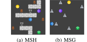 Figure 2. Overview of Markov Stag-Hunt and Markov Snowdrift. There are four agents, repre- sented by colored circles, in each paradigm. (a) Agents catch prey for reward. A stag with a reward of 10 requires at least two agents to hunt together. One agent can hunt a hare with a reward of 1. (b) Everyone gets a reward of 6 when an agent removes a snowdrift. When a snowdrift is removed, removers share the cost of 4 evenly
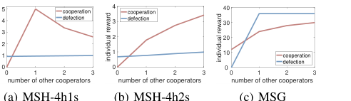 Figure 3. Schelling diagrams for (a) MSH-4h1s, (b) MSH-4h2s, and (c) MSG
Results, Limitations & Conclusion
Experimental Design & Baselines
To rigorously validate the Hierarchical Opponent modeling and Planning (HOP) algorithm, the authors conducted experiments across two distinct mixed-motive environments: the Markov Stag-Hunt (MSH) and the Markov Snowdrift Game (MSG). These environments are spatial and temporal extensions of classic game theory paradigms, designed to elicit complex strategic interactions.
In MSH, four agents hunt prey (stags and hares) on a grid. A stag provides a reward of 10 but requires at least two agents to hunt cooperatively, splitting the reward. A hare provides a reward of 1 and can be caught by a single agent. The game ends after 30 timesteps. Two MSH settings were used:
- MSH-4h1s: Features four hares and one stag. This setup encourages cooperation for the stag while maintaining competition for hares, creating a mixed-motive dynamic.
- MSH-4h2s: Includes four hares and two stags. This increases the potential for cooperation but introduces a twist: the game terminates just five timesteps after the first successful hunt, intensifying the tension between immediate individual gain and long-term collective benefit.
The MSG environment places six snowdrifts randomly on an 8x8 grid. Agents can move, stay idle, or "remove a snowdrift." Removing a snowdrift incurs a shared cost of 4 among removers, but each agent receives an individual reward of 6. The core dilemma here is free-riding: an agent can get a higher reward by letting others remove snowdrifts. The game concludes when all snowdrifts are cleared or after 50 timesteps. In both MSH and MSG, four agents operate without direct communication or access to each other's internal parameters. Schelling diagrams were employed to visually confirm that these environments effectively capture the inherent dilemmas of mixed-motive interactions, where optimal strategies shift based on co-players' behavior.
The "victims" (baseline models) against which HOP was tested included a diverse set of established multi-agent reinforcement learning (MARL) algorithms and rule-based strategies:
- Learning Baselines: LOLA (Learning with Opponent-Learning Awareness), SI (Social Influence), A3C (Asynchronous Advantage Actor-Critic), PS-A3C (Prosocial A3C), PR2, and direct-OM (an ablated version of HOP that models co-players directly with neural networks without goal conditioning).
- Rule-Based Baselines: Random (takes valid actions randomly), Cooperator (consistently adopts cooperative behavior), and Defector (consistently adopts exploitative behavior).
The experimental validation proceeded in two phases:
1. Self-play: All agents using the same algorithm were trained until their performance converged. This phase assessed the algorithm's ability to make autonomous decisions and achieve cooperation in mixed-motive settings.
2. Few-shot Adaptation: A focal HOP agent interacted with three co-players running different baseline algorithms for 2400 steps. The focal agent's average reward during the final 600 steps was used to quantify its adaptation ability. Policy parameters could be updated during this phase if the algorithm supported it.
To provide a clear reference for optimal performance, an "Orcale agent" was trained for each co-player type. This Orcale agent, trained via A3C with fixed co-player parameters over extensive interactions, represents the best possible performance an agent could achieve when perfectly adapted to a specific co-player. All rewards were min-max normalized between the Orcale agent's performance (optimal) and the random policy's performance (lowest), allowing for a standardized comparison.
What the Evidence Proves
The experimental results definitively demonstrate HOP's superior capabilities in both self-play and few-shot adaptation within mixed-motive environments, ruthlessly proving its core mathematical claims regarding hierarchical opponent modeling and planning.
In **self-play scenarios
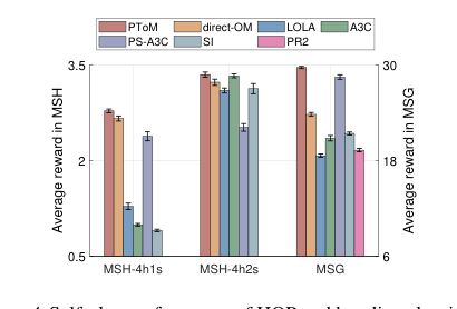 Figure 4. Self-play performance of HOP and baseline algorithms. Shown is the average reward in the self-play training phase
**, HOP consistently achieved high rewards, often outperforming or matching the best baselines. In MSH-4h1s, HOP, direct-OM, and PS-A3C learned to hunt stags, but PS-A3C's "lazy agent" problem led to inferior rewards. LOLA exhibited unstable strategies, while SI and A3C primarily hunted hares, yielding low returns. PR2 failed entirely in MSH. In MSH-4h2s, HOP and A3C were the most stable and yielded the highest returns, successfully coordinating for stag hunts. Most notably, in MSG, HOP achieved the highest reward, closely approaching the theoretical optimum of 30.0. This highlights HOP's strong propensity for cooperation in a decentralized setting, contrasting with baselines like LOLA, A3C, and SI, which prioritized individual profits and struggled with coordination. PS-A3C, while second best, still faced coordination issues when only one snowdrift remained.
The most compelling evidence for HOP's core mechanism lies in its few-shot adaptation performance (Table 1). HOP consistently achieved the "overall best adaptation percentage" in most test scenarios: 83.3% in MSH-4h1s, a perfect 100.0% in MSH-4h2s, and 83.3% in MSG. This far surpassed other algorithms, which only achieved optimal adaptation in specific, limited scenarios where co-player behavior aligned with their pre-learned policies.
The paper provides a clear example of how HOP's belief update mechanism works in reality **
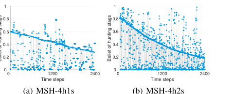 Figure 5. Visualization of HOP’s belief in adaptation to three de- fectors in MSH. Every blue-filled circle represents HOP’s inferred probability (i.e., belief) that a co-player hunts stags
. When facing three defectors (who consistently hunt hares) in MSH, HOP initially held a "false belief" that co-players would hunt stags (a bias from its self-play experience). However, the intra-OM module (updating beliefs within an episode) quickly corrected this. By observing co-players' trajectories (e.g., moving towards a hare), intra-OM inferred their true goal, leading to accurate opponent models. The inter-OM module** (updating beliefs across episodes) further accelerated this convergence to the true belief, acting as a precise prior for subsequent episodes. The declining line in Figure 5, representing the gradual reduction of the prior belief in stag hunting, is definitive, undeniable evidence that HOP's hierarchical belief updating mechanism effectively adapts to unseen and dynamic co-player behaviors. With these accurate co-player policies as input, the planning module could then compute advantageous actions, allowing HOP to make substantial strategic adjustments and achieve high returns even against non-cooperative agents like defectors.
Furthermore, the experiments revealed the emergence of social intelligence (Appendix G, Figure 6) among multiple HOP agents. In one instance, "self-organized cooperation" emerged where four HOP agents collectively hunted a stag for a higher total reward, even though it was individually riskier than hunting hares. This occurred through independent decision-making, with agents inferring each other's intentions and coordinating without centralized control. In another case, "alliance of the disadvantaged," two less greedy HOP agents successfully misled a greedier co-player to avoid collaboration, then cooperated to maximize their own profits. These observations underscore that HOP's ability to infer others' goals and rapidly adjust its responses facilitates complex social behaviors, even when agents are self-interested.
Limitations & Future Directions
While HOP demonstrates remarkable prowess in few-shot adaptation within mixed-motive environments, the authors candidly acknowledge several limitations that pave the way for exciting future research.
Firstly, a significant constraint is the requirement for a clear definition of goals within any given environment for HOP to function effectively. The current framework relies on pre-defined goal sets. To enhance HOP's generalizability and applicability across a wider array of complex scenarios, a crucial future direction involves developing techniques that can autonomously abstract goal sets. This would allow HOP to operate in novel environments without manual intervention, a challenge that some prior work has begun to explore.
Secondly, the current implementation of HOP utilizes a Level-0 Theory of Mind (ToM), which essentially involves an agent reasoning about "what they think." While effective, incorporating higher-order ToM, such as Level-1 ToM ("what I think they think about me"), holds the potential to significantly improve predictions about co-players' behaviors. However, this comes with a substantial increase in computational cost due to the nested belief inference involved. Therefore, future work must focus on developing advanced and computationally efficient planning methods that can effectively and rapidly leverage the richer insights provided by higher-order ToM without succumbing to prohibitive computational complexity. This is a non-trivial engineering and mathematical hurdle.
Thirdly, although the paper selected a diverse set of well-established algorithms as co-players for evaluation, none of them fully capture the nuances and complexities of human behavior. The ultimate goal of many multi-agent systems is to interact seamlessly with human participants. Consequently, a compelling future research avenue is to explore HOP's performance in few-shot adaptation scenarios involving actual human participants. This would provide invaluable insights into its real-world applicability and robustness.
Finally, a critical discussion point arises from HOP's inherent self-interested nature. While it excels at maximizing its own returns, this does not always guarantee alignment with the best interests or values of human co-players. To mitigate this potential misalignment and foster more beneficial human-AI collaboration, future research should investigate how HOP's powerful inference capabilities can be leveraged to infer and optimize for human values and preferences during interactions. This could involve incorporating mechanisms for value alignment or preference learning, allowing HOP to assist humans in complex environments in a way that is not only efficient but also ethically sound and socially beneficial. This would require a deep dive into human-AI interaction ethics and robust preference elicitation techniques.
 Table 5. Performance of HOP and its ablation versions in MSH-4h2s. In (a) self-play, 4 agents of the same kind are trained to converge. Shown is the normalized score after convergence. In (b) few-shot adaptation, the interaction happens between 1 agent using the row policy and 3 co-players using the column policy. Shown are the min-max normalized scores, with normalization bounds set by the rewards of Orcale and the random policy. The results are depicted for the row policy from 1800 to 2400 step