Highway Value Iteration Networks

Background & Academic Lineage

The Origin & Academic Lineage

The core of this research stems from the long-standing challenge of enabling artificial intelligence agents to perform effective long-term planning. This specific problem first emerged prominently with the advent of Value Iteration Networks (VINs), introduced by Tamar et al. in 2016. VINs were a significant step forward because they integrated a "planning module" directly into a neural network (NN) architecture, allowing for end-to-end learning of planning tasks. This planning module was designed to approximate the classical value iteration algorithm, a fundamental concept in reinforcement learning (RL) formalized by Bellman in 1966.

Historically, while VINs showed remarkable proficiency in various planning tasks like path planning and autonomous navigation, they faced a critical limitation: their ability to handle long-term planning. As the complexity of tasks increased, requiring more planning steps (e.g., path lengths exceeding 120 in a maze), the sucess rate of VINs drastically declined, often falling below 10%. A natural approach to improve long-term planning is to increase the depth of the VIN's planning module, allowing it to simulate more planning steps. However, this immediately ran into a fundamental problem in deep learning: training very deep neural networks is inherently difficult due to issues like vanishing or exploding gradients (Hochreiter, 1991). While techniques like residual networks and highway networks had successfully enabled the training of very deep NNs for classification tasks, these methods had not proven equally effective when applied to the unique architecure of VINs, particularly in planning contexts. This disparity arises because VINs incorporate a specific inductive bias from reinforcement learning, which is grounded in the theoretically sound value iteration algorithm. The authors were thus compelled to develop a new approach that could effectively train deep VINs for long-term planning by integrating advanced techniques from both NNs and RL.

Intuitive Domain Terms

To help a zero-base reader grasp the concepts, here are some specialized terms translated into everyday analogies:

• Value Iteration Network (VIN): Imagine a smart GPS that not only tells you the best route but also learns how to find the best route by repeatedly simulating all possible future steps and their outcomes, much like you'd mentally "iterate" through options to find the most valuable one. A VIN is a neural network with this kind of built-in "thinking ahead" module.
• Long-term Credit Assignment: Think of teaching a dog a complex trick that involves many steps. If the dog finally gets a treat at the very end, it's hard for the dog to know which specific earlier actions contributed to getting the treat. In AI, long-term credit assignment is the challeng of figuring out which actions, taken many steps ago, were truly responsible for a good (or bad) outcome much later.
• Vanishing/Exploding Gradients: Imagine playing a game of "telephone" with a very long line of people. If the message is whispered too softly (vanishing gradient), it gets lost by the end. If it's shouted too loudly (exploding gradient), it becomes distorted noise. In deep learning, gradients are like the "feedback" signal that tells the network how to adjust its internal settings. If this feedback gets too weak or too wild across many layers, the network can't learn effectively.
• Skip Connections: Imagine a very long, winding road. Skip connections are like adding direct shortcuts or express lanes that bypass some of the winding parts. This allows information (or the "feedback" signal for learning) to travel more easily and directly across many layers of a neural network, preventing it from getting lost or diluted along the way.

Notation Table

Notation	Description	Category
$s$	A specific state in the environment.	Variable
$a$	An action taken by the agent.	Variable
$V^\pi(s)$	The value function, representing the expected total future reward from state $s$ when following policy $\pi$.	Variable
$Q^\pi(s, a)$	The action-value function, representing the expected total future reward from state $s$ when taking action $a$ and then following policy $\pi$.	Variable
$V^{(n)}$	The value function at the $n$-th iteration of the value iteration algorithm.	Variable
$\gamma$	The discount factor, a value between 0 and 1 that determines the importance of future rewards.	Parameter
$N$	The total depth (number of layers) of the neural network.	Parameter
$N_B$	The number of "highway blocks" in the network architecture.	Parameter
$N_p$	The number of parallel Value Exploration (VE) modules within a highway block.	Parameter
$\epsilon$	The exploration rate, controlling the randomness in action selection during training.	Parameter

Problem Definition & Constraints

Core Problem Formulation & The Dilemma

The core problem this paper addresses is the significant challenge of enabling Value Iteration Networks (VINs) to perform effective long-term planning.

Input/Current State:
The current state involves Value Iteration Networks (VINs), which are neural network architectures designed for end-to-end learning in planning tasks. VINs achieve this by embedding a differentiable "planning module" that approximates the classic value iteration algorithm. These networks have demonstrated considerable proficiency in various planning scenarios, such as path planning and autonomous navigation, particularly for tasks requiring a relatively limited number of planning steps.

Desired Endpoint/Goal State:
The desired goal is to develop VINs capable of robust and accurate long-term planning. This means the networks should be able to handle tasks that necessitate hundreds of planning steps, such as navigating complex mazes with very long shortest paths. Crucially, these advanced VINs should be trainable to significant depths (hundreds of layers) using standard backpropagation techniques, maintaining high success rates even for extended planning horizons.

Missing Link & Mathematical Gap:
The exact missing link is the inability of existing VIN architectures to scale effectively to deep network configurations required for long-term planning. While deeper planning modules should allow for more planning steps and thus better long-term performance, current VINs encounter severe difficulties when their depth increases.

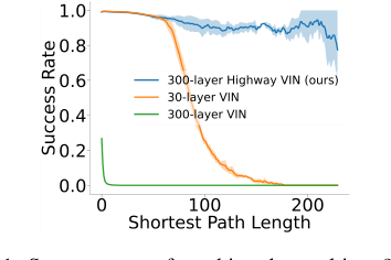Figure 1. Success rates of reaching the goal in a 25 × 25 maze problem. The success rate of a 30-layer VIN con- siderably decreases as the shortest path length increases, and training a 300-layer VIN is difficult and exhibits poor performance

Figure 1 starkly illustrates this: a 30-layer VIN's success rate plummets for shortest path lengths exceeding 120, and attempting to train a 300-layer VIN proves difficult, resulting in poor performance. The mathematical gap lies in designing a VIN architecture that can propagate information and gradients effectively through hundreds of layers, allowing the embedded value iteration process to converge to an optimal value function over many iterations without succumbing to the inherent challenges of deep learning.

The Painful Trade-off or Dilemma:
The central dilemma trapping previous researchers is the inherent conflict between the need for depth in planning and the practical limitations of training deep neural networks. On one hand, a deeper planning module within a VIN is theoretically desirable as it allows for a greater number of iterative planning steps, which is essential for solving long-term planning problems. On the other hand, increasing the depth of any neural network, including VINs, typically introduces severe complications such as vanishing or exploding gradients. While general deep learning has developed techniques (like skip connections in ResNets or DenseNets) to train very deep networks for classification, these methods have not been "equally successful in planning tasks" for VINs. This disparity suggests that the unique inductive bias of VINs, derived from the value iteration algorithm in reinforcement learning, makes them particularly susceptible to these depth-related training issues, creating a painful trade-off between architectural depth for planning capability and practical trainability.

Constraints & Failure Modes

The problem of achieving long-term planning with deep VINs is insanely difficult due to several harsh, realistic constraints and failure modes:

1. Computational Constraint: Vanishing/Exploding Gradients: The most fundamental hurdle is the well-known vanishing or exploding gradient problem in deep neural networks. As the paper states, "increasing the depth of an NN can introduce complications, such as vanishing or exploding gradients, which is a fundamental problem in deep learning." This makes it exceedingly hard to train VINs with hundreds of layers effectively using standard backpropagation, as gradients either become too small to update early layers or too large, leading to unstable training.

2. Architectural Constraint: Incompatibility with Standard Deep Learning Solutions: While skip connections (e.g., in Highway Networks, ResNets, DenseNets) have proven effective for training very deep networks in other domains (like image classification), they haven't translated well to VINs for planning tasks. This suggests a specific architectural incompatibility or a lack of appropriate inductive bias in these general-purpose deep learning techniques when applied to the planning module of VINs, which is grounded in reinforcement learning's value iteration.

3. Performance Failure Mode: Degradation with Depth: Instead of improving, the performance of VINs drastically degrades with increased depth for long-term planning. For instance, VINs with depths greater than 150 layers show a success rate of nearly 0% for many tasks. This is a critical failure mode where the intended solution (more depth for more planning steps) actively worsens the outcome.

4. Information Flow Constraint: Greedy Action Selection & Gradient Channeling: The original VIN's value iteration module "greedily takes the largest Q value" (Eq. 4). This mechanism creates a "distinctive information flow for each layer, thereby channeling gradients toward certain specific neurons." This lack of diverse information and gradient flow across spatial dimensions makes it difficult for the network to learn robustly and generalize across complex, long-term planning scenarios.

5. Exploration Failure Mode: Detrimental Stochasticity: While introducing stochasticity (exploration) can help diversify information flow, uncontrolled exploration can be counterproductive. The paper notes that without a "filter gate" to manage exploration, "highway VINs could easily suffer the adverse effects of exploration in VE modules, which could prevent convergence." This implies that naive attempts to improve diversity can lead to instability and prevent the network from learning an optimal policy.

6. Hardware Memory Limits: Although not the primary focus of the problem definition, the computational complexity of very deep networks imposes practical hardware memory limits. The paper's experimental section (Table 4) shows that the proposed Highway VIN, while more efficient than some alternatives, still requires 15.0G of GPU memory for a 300-layer network, compared to 3.1G for a 30-layer VIN. This indicates that scaling to even deeper architectures or larger problem sizes would quickly hit memory ceilings, making research and deployment more expensive and difficult.

Why This Approach

The Inevitability of the Choice

The adoption of the highway value iteration network (highway VIN) was not merely a choice but an inevitability driven by the inherent limitations of existing approaches when confronted with the demands of long-term planning. The authors pinpointed the exact moment of insufficiency for traditional methods when observing Value Iteration Networks (VINs) in path planning tasks. Specifically, for shortest path lengths exceeding 120, the success rate of VINs plummeted below 10% (Figure 1). This stark decline highlighted a fundamental flaw: while increasing the depth of VIN's embedded "planning module" seemed a logical path to integrate more planning steps and thus improve long-term planning, traditional deep neural network (NN) training complications, such as vanishing or exploding gradients, quickly rendered this approach unviable.

Crucially, the paper notes that even advanced deep NNs, which have successfully tackled these gradient issues in classification tasks (e.g., ResNets, DenseNets, and standard Highway Networks), were not equally successful in planning tasks (Table 1, Section 5). This disparity arises directly from the unique architecture of VINs and their intrinsic inductive bias derived from the value iteration algorithm in reinforcement learning (RL). Standard deep NN solutions, while effective for general deep learning, simply do not provide the specific RL-relevant prior knowledge necessary to facilitate efficient long-term credit assignment within the VIN's planning framework. Therefore, a solution that could both enable deep architectures and preserve/enhance the VIN's planning inductive bias was the only viable path forward, leading to the integration of highway value iteration and architectural innovations like skip connections tailored for this specific problem.

Comparative Superiority

The highway VIN demonstrates qualitative superiority over previous gold standards not just through improved performance metrics, but via a fundamental structural redesign that addresses the core challenges of deep planning. Its overwhelming advantage stems from three key innovations embedded within the VIN's planning module:

1. Aggregate Gate: This component constructs skip connections, significantly improving information flow across many layers. Unlike generic skip connections in standard highway networks, this is integrated within the value iteration context, enabling the training of VINs with hundreds of layers without suffering from vanishing or exploding gradients. This structural advantage directly facilitates the deep architectures required for long-term planning.
2. Exploration Module: This module injects controlled stochasticity during training, which diversifies information and gradient flow across spatial dimensions. This is a critcal improvement over traditional VINs, where the greedy maximization operation in the value iteration module can lead to limited diversity in selected actions, as evidenced by the low entropy values for VINs compared to highway VINs (Table 2). This diversity is essential for robust learning in complex, high-dimensional planning environments.
3. Filter Gate: Designed to "filter out" useless exploration paths, this gate ensures safe and efficient exploration. It compares activations and discards those that do not contribute to convergence, a mechanism crucial for maintaining the theoretical soundness of value iteration, especially when combined with the stochasticity introduced by the exploration module. Without this, as ablation studies show (Figure 7), the perfomance drastically decreases, as the network would suffer from adverse effects of unguided exploration.

These components collectively allow highway VINs to learn more effective value functions for states distant from the goal (Figure 6), implying a superior ability to handle long-term dependencies and plan over extended horizons, a capability severely lacking in traditional VINs and other deep NNs in planning tasks.

Alignment with Constraints

The chosen highway VIN approach perfectly aligns with the harsh requirements of long-term planning, forming a "marriage" between the problem's demands and the solution's unique properties.

One primary constraint is the necessity for deep networks to perform long-term planning, as more planning steps inherently require greater depth. Traditional VINs failed here due to training difficulties at increased depths. Highway VIN directly addresses this by enabling effective training with hundreds of layers using standard backpropagation, a feat impossible for its predecessors.

Another critical constraint is overcoming the vanishing or exploding gradient problem inherent in very deep NNs. The aggregate gate, by introducing skip connections, directly tackles this, ensuring stable gradient flow. This is a direct adaptation of proven deep learning techniques (like those in highway networks and ResNets) but specifically integrated into the VIN architecture to preserve its planning inductive bias.

Furthermore, the problem demands efficient long-term credit assignment within the RL framework. The very foundation of this approach, highway value iteration, was designed precisely for this purpose (Wang et al., 2024). The integration of this algorithm ensures that the solution is theoretically sound and converges to the optimal value function (Remark 1), even with the added stochasticity of the exploration module, thanks to the filter gate (Remark 2). This ensures that the deep network is not just "deep" but effectively deep for planning.

Rejection of Alternatives

The paper provides clear reasoning for rejecting other popular or state-of-the-art approaches for this specific problem:

1. Traditional VINs: These are explicitly shown to be insufficient for long-term planning. As depth increases beyond a certain point (e.g., 30 layers for a 25x25 maze), their success rate drastically drops, often to below 10% for path lengths over 120 (Figure 1, Table 1). The difficulty in training very deep VINs due to gradient issues makes them unsuitable for tasks requiring hundreds of planning steps.

2. Standard Deep Neural Networks (e.g., Highway Networks, ResNets, DenseNets): While these architectures excel in tasks like image classification by enabling the training of very deep models, they are not "equally successful in planning tasks" (Page 1). The authors hypothesize that simply integrating their skip connections into VINs does not introduce the additional architectural inductive bias beneficial for planning (Page 8). These methods, lacking the specific RL-relevant inductive bias of value iteration, fail to translate their depth into improved long-term planning capabilities. Table 1 clearly shows that while highway networks maintain performance at greater depths than VINs, their long-term planning capabilities do not significantly improve with increased depth, and they are still outperformed by highway VINs.

3. Gated Path Planning Networks (GPPNs): GPPNs, a recurrent variant of VINs, were designed to improve training stability in deep models. While they perform robustly and excel in short-term planning tasks (e.g., 99.09% SR for SPL [1,30] in a 25x25 maze), their performance significantly degrades for long-term planning, dropping to less than 3% for SPLs [130,230] (Table 1, Page 8). The paper attributes this failure to GPPN being a "black box method with less inductive bias towards planning," making it more suited for learning short-term patterns rather than true long-term planning skills. This highlights that a strong, explicit planning inductive bias, as provided by highway value iteration, is crucial.

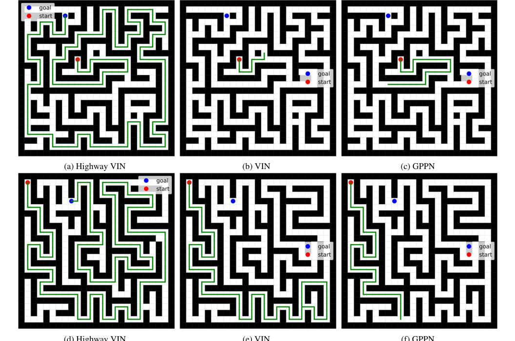Figure 11. Examples of 2D maze navigation tasks where highway VIN succeeds, but other methods fail

Mathematical & Logical Mechanism

The Master Equation

The core of the Highway Value Iteration Networks (Highway VINs) lies in its "planning module," which is designed to approximate the Highway Value Iteration (highway VI) algorithm. The central mathematical engine driving this algorithm is the $G$ operator, which defines how the value function is updated iteratively. The paper states that the highway VI algorithm iteratively updates the value function as $V^{(n+1)} = GV^{(n)}$, where $G$ is formally defined as:

$$ GV(s) = \max_{\Pi \in \mathbf{\Pi}} \max_{N \in \mathbf{N}} \max_{a \in \mathcal{A}} \max_{x \in \mathcal{X}} \{(B^{\pi})^{\circ(N-1)} BV, BV\} $$

This equation encapsulates the multi-step bootstrapping and policy exploration mechanisms that are fundamental to highway VI and, by extension, to the Highway VIN architecture.

Term-by-Term Autopsy

Let's dissect this master equation to understand each component's role and meaning.

• $GV(s)$:

  • Mathematical Definition: This represents the updated value function for a given state $s$ after applying the Highway Value Iteration operator $G$.
  • Physical/Logical Role: It's the new, improved estimate of the optimal value achievable from state $s$, incorporating insights from multiple planning horizons and policies. This is the output of one "highway block" iteration in the VIN's planning module.
  • Why this operator: The $G$ operator is a composite operator designed to facilitate efficient long-term credit assignment in reinforcement learning, combining elements of both optimal and policy-based value iteration.

• $V(s)$:

  • Mathematical Definition: The current estimate of the value function for state $s$. In the iterative update $V^{(n+1)} = GV^{(n)}$, this would be $V^{(n)}(s)$.
  • Physical/Logical Role: This is the input to the $G$ operator, representing the agent's current understanding of how good each state is. It's the foundation upon which the next, more refined value estimate is built.

• $\max_{\Pi \in \mathbf{\Pi}}$:

  • Mathematical Definition: A maximization operation over a set of policies.
  • Physical/Logical Role: This term allows the algorithm to consider and select the best "lookahead policy" from a predefined set $\mathbf{\Pi}$. It ensures that the planning process is not restricted to a single, fixed policy but can explore different strategies to find the most promising path. This is a key aspect of the "exploration module" in Highway VINs.
  • Why maximization: Maximization is used here to select the most optimistic outcome among different potential planning strategies, aligning with the goal of finding an optimal value function.

• $\mathbf{\Pi}$:

  • Mathematical Definition: A set of lookahead policies.
  • Physical/Logical Role: These are the various policies that the agent can "imagine" or "simulate" to explore future states and rewards. In the Highway VIN, these correspond to the embedded policies within the Value Exploration (VE) modules.

• $\max_{N \in \mathbf{N}}$:

  • Mathematical Definition: A maximization operation over a set of lookahead depths.
  • Physical/Logical Role: This allows the algorithm to consider different "planning horizons" or how many steps into the future it should look. It's crucial for long-term planning, as it enables the model to choose the most beneficial depth of planning for a given situation.
  • Why maximization: Similar to policies, maximizing over depths helps select the most advantageous planning horizon, ensuring the algorithm can adapt its planning scope.

• $\mathbf{N}$:

  • Mathematical Definition: A set of lookahead depths.
  • Physical/Logical Role: These are the different numbers of steps (or iterations) that the planning module can simulate into the future. The paper mentions $n$ as the lookahead depth, so $N$ here refers to the specific depth chosen from the set $\mathbf{N}$.

• $\max_{a \in \mathcal{A}}$:

  • Mathematical Definition: A maximization operation over the set of possible actions.
  • Physical/Logical Role: This term ensures that at each decision point, the algorithm considers all available actions and selects the one that leads to the highest expected value. This is a fundamental part of value iteration.
  • Why maximization: This is the core of the Bellman optimality principle, aiming to find the best possible action to maximize future rewards.

• $\mathcal{A}$:

  • Mathematical Definition: The set of all possible actions an agent can take.
  • Physical/Logical Role: These are the discrete choices available to the agent in its environment.

• $\max_{x \in \mathcal{X}}$:

  • Mathematical Definition: A maximization operation over the set of states or spatial locations.
  • Physical/Logical Role: This implies that the operator considers the best possible outcome across different spatial configurations or states, which is relevant in maze navigation tasks where the "state" might be a grid cell.
  • Why maximization: This ensures the algorithm is robust to different starting points or local variations in the environment, always aiming for the globally optimal path.

• $B$:

  • Mathematical Definition: The Bellman optimality operator. For a state $s$, $BV(s) = \max_a \sum_{s'} T(s'|s,a) [R(s,a,s') + \gamma V(s')]$.
  • Physical/Logical Role: This operator calculates the optimal value of a state by considering the immediate reward and the discounted value of the next state, assuming the agent always takes the best action. It represents a "greedy" planning step. In the Highway VIN, this is approximated by the standard Value Iteration (VI) module (Eq. 3 and 4).
  • Why summation and maximization: Summation is used to average over possible next states (weighted by transition probabilities), while maximization selects the best action.

• $B^\pi$:

  • Mathematical Definition: The Bellman expectation operator for a given policy $\pi$. For a state $s$, $B^\pi V(s) = \sum_a \pi(a|s) \sum_{s'} T(s'|s,a) [R(s,a,s') + \gamma V(s')]$.
  • Physical/Logical Role: This operator calculates the expected value of a state under a specific policy $\pi$. It represents a "policy-driven exploration" step. In the Highway VIN, this is approximated by the Value Exploration (VE) module (Eq. 6 and 7), which injects stochasticity.
  • Why summation: Summation is used twice: once to average over actions (weighted by policy probabilities) and again to average over possible next states.

• $\circ(N-1)$:

  • Mathematical Definition: The composition operator, applied $N-1$ times. For an operator $O$, $O^{\circ k} = O \circ O \circ \dots \circ O$ ($k$ times). The paper uses $n-1$ in Eq. (5), but given that $N$ is defined as lookahead depth, it's more consistent to interpret this as $N-1$ compositions.
  • Physical/Logical Role: This signifies multi-step lookahead. Applying the Bellman expectation operator multiple times means simulating the policy $\pi$ for $N-1$ steps into the future. This allows the algorithm to evaluate the long-term consequences of a policy, not just the immediate next step. In the Highway VIN, this corresponds to stacking $N_b-1$ parallel VE modules.
  • Why composition: Composition naturally represents sequential application of an operator, modeling multi-step planning.

• $\{\cdot, \cdot\}$:

  • Mathematical Definition: A set containing two elements.
  • Physical/Logical Role: This indicates that the $G$ operator considers two main branches of value propagation: one that involves multi-step policy-based exploration ($(B^{\pi})^{\circ(N-1)} BV$) and another that represents a more direct, single-step optimal update ($BV$). The outer maximization then chooses the better of these two. This is where the "filter gate" comes into play, selecting the maximum value.
  • Why set and outer maximization: This structure allows for a comparison between a deep, explorative path and a more immediate, greedy path, ensuring that the algorithm benefits from both short-term optimality and long-term exploration.

Step-by-Step Flow

Imagine a single abstract data point, representing the value of a state $V^{(n)}(s)$, entering the Highway VIN's planning module. This module acts like a sophisticated assembly line, processing $V^{(n)}(s)$ to produce an improved $V^{(n+1)}(s)$.

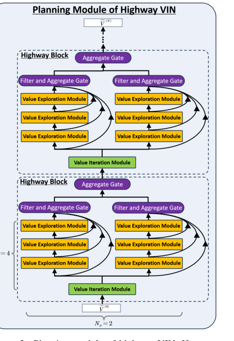Figure 3. Planning module of highway VIN. Here, we demonstrate the planning module of highway VIN using a highway block of depth Nb = 4 and incorporating Np = 2 embedded policies

1. Initial Input: The current value function estimate, $V^{(n)}(s)$, is fed into the planning module. This $V^{(n)}(s)$ is typically a feature map representing the value of each spatial location in the latent MDP.

2. Bellman Optimality Path (The "Greedy" Lane):

   • A portion of $V^{(n)}(s)$ is directed to a standard Value Iteration (VI) module.
   • Inside this module, a convolutional operation (like in Eq. 3) computes action-values $Q_{a,i,j}^{(n)}$ by considering immediate rewards and the discounted values of neighboring states.
   • A max-pooling operation (Eq. 4) then selects the maximum $Q_{a,i,j}^{(n)}$ over all actions $a$ for each state $(i,j)$, effectively applying the Bellman optimality operator $B$. This yields an updated value function, let's call it $V_{VI}^{(n+1)}(s) = BV^{(n)}(s)$. This path represents the most direct, greedy update.

3. Bellman Expectation Path (The "Exploration" Lanes):

   • Simultaneously, $V^{(n)}(s)$ is also routed to multiple parallel Value Exploration (VE) modules. Each VE module is associated with a different "lookahead policy" $\pi_{np}$ and contributes to a specific "lookahead depth" $n_b$.
   • Within each VE module: Instead of taking a maximum over actions, the VE module computes an expected value over actions based on its embedded policy $\pi_{np}$ (Eq. 7). This policy can be generated stochastically during training (Eq. 8), injecting diversity. This effectively applies the Bellman expectation operator $B^{\pi_{np}}$.
   • Stacking for Depth: These VE modules are stacked for $N_b - 1$ layers. This means the output of one VE module becomes the input to the next, composing the $B^{\pi_{np}}$ operator multiple times, resulting in $(B^{\pi_{np}})^{\circ(n_b-1)} BV^{(n)}(s)$ for various $n_b$ and $np$. This creates a rich set of explorative value estimates, considering different policies and planning horizons.

4. Aggregation (The "Information Merge"):

   • The outputs from all these parallel and stacked VE modules, along with the output from the VI module, converge.
   • An "aggregate gate" (like Eq. 9) combines these diverse activations. This gate uses learnable softmax weights to determine the contribution of each parallel VE module and each depth to the final aggregated value. This creates skip connections, allowing information to flow across many layers and depths, mitigating vanishing gradients.

5. Filtering (The "Quality Control"):

   • After aggregation, a "filter gate" applies a maximization operation. This gate compares the aggregated value (which represents a potential exploration path) with a more direct, often greedy, value (e.g., $V^{(n+1)}$ from the VI module or a previous iteration's value).
   • It selects the maximum of these values, effectively discarding "useless exploration paths" that do not contribute to convergence or lead to lower values. This ensures that only beneficial information is propagated forward.

6. Output: The result of this entire process, after aggregation and filtering, becomes the new, refined value function estimate, $V^{(n+1)}(s)$ (or $V^{(n+N_b)}(s)$ in the paper's notation for a highway block). This output then feeds into the next highway block or is used to derive the final policy.

This intricate dance of parallel processing, policy-driven exploration, and selective aggregation allows the Highway VIN to perform robust, long-term planning.

Optimization Dynamics

The Highway VIN learns and converges through an end-to-end training process, primarily leveraging standard backpropagation, but with specific architectural innovations designed to shape the loss landscape and gradient flow.

1. Differentiable Planning Module: The entire planning module, including the Value Iteration (VI) modules, Value Exploration (VE) modules, aggregate gates, and filter gates, is designed to be fully differentiable. This is crucial because it allows gradients to flow backward through the planning steps, enabling the network to learn how to plan.

2. Backpropagation and Gradient Flow: The model is trained using standard backpropagation. A loss function (e.g., based on imitation learning, comparing predicted policies/values to target policies/values) is computed at the output layer. Gradients of this loss are then propagated backward through all layers of the network, including the deep planning module, to update the model's parameters.

3. Addressing Vanishing/Exploding Gradients: The primary motivation for Highway VIN is to overcome the vanishing/exploding gradient problem in very deep networks, especially in planning tasks.

   • Aggregate Gate (Skip Connections): The aggregate gate explicitly introduces skip connections, similar to highway networks and ResNets. These connections provide direct pathways for gradients to flow from later layers to earlier layers, bypassing multiple non-linear transformations. This helps to maintain strong gradient signals even in very deep architectures, making training hundreds of layers feasible.
   • Value Exploration Module (Stochasticity): The VE module injects controlled stochasticity during training by randomly generating embedded policies (Eq. 8). This diversifies the information and gradient flow across spatial dimensions. While stochasticity can sometimes hinder convergence, the paper notes that this mechanism improves robustness and is essential for high performance without impacting convergence to the optimal value function (Remark 1). This suggests it helps explore the loss landscape more effectively, preventing the model from getting stuck in poor local minima.

4. Shaping the Loss Landscape (Convergence Guarantees):

   • Filter Gate (Maximization): The filter gate, which performs a maximization operation, is explicitly stated as "crucial for ensuring convergence to $V^*$." (Remark 2). By discarding "useless exploration paths" (i.e., activations that are lower than a more direct value), it prunes away suboptimal branches of the planning process. This effectively shapes the loss landscape by guiding the model towards regions that lead to optimal value functions, preventing divergence due to unhelpful explorations.
   • Theoretical Soundness: The underlying highway VI algorithm is proven to converge to the optimal value function $V^*$ regardless of the specific lookahead policies, depths, or softmax temperatures (Remark 1). This theoretical guarantee provides a strong foundation for the Highway VIN's learning dynamics, suggesting that the iterative updates, when properly filtered, will eventually lead to an optimal solution.

5. Learnable Parameters: The model learns by updating several sets of parameters:

   • The weights of the convolutional layers in the VI and VE modules.
   • The learnable parameters $W_{np}^{(n+n_b)}$ used to generate the embedded policies in the VE modules.
   • The softmax temperatures $\alpha_a^{(n_p+n_b)}$ and $\alpha_n^{(n_p+n_b)}$ in the aggregate gates, which control the weighting of different information paths.

Through this combination of architectural design, controlled stochasticity, and theoretically grounded operators, the Highway VIN effectively learns to perform long-term planning by iteratively refining its value function estimates, overcoming the challenges of deep network training in complex sequential decision-making tasks.

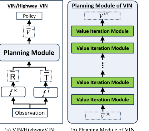Figure 2. (a): Architecture of VIN and highway VIN. (b): Architecture of the planning module of VIN, which includes N layers of value iteration modules. The architecture of the value iteration module is detailed in Fig. 4(a)

Results, Limitations & Conclusion

Experimental Design & Baselines

To rigorously validate their claims, the authors conducted a series of experiments primarily focused on 2D maze navigation and, to a lesser extent, 3D ViZDoom navigation tasks. The experimental setup for 2D maze navigation closely followed that described in the GPPN paper (Lee et al., 2018). For these tasks, agents were trained to navigate mazes of varying sizes, specifically $15 \times 15$ and $25 \times 25$, with actions including moving forward, turning 90 degrees left or right, and maintaining four orientations.

The training regimen involved 30 epochs of imitation learning on labeled datasets, comprising 25K mazes for training, 5K for validation, and 5K for testing. The RMSprop optimizer was used with a learning rate of 0.001 and a batch size of 32. Convolutional operations within the planning module utilized a kernel size of 5, and the neural network mapping observations to the latent MDP had a hidden dimension of 150.

The primary metric for evaluating planning ability was the success rate (SR), defined as the ratio of successfully completed tasks to the total number of planning tasks. A task was considered successful if the agent generated a path from the start to the goal within a predefined number of steps. To assess long-term planning capabilities, algorithms were evaluated across tasks with varying shortest path lengths (SPLs), pre-calculated using Dijkstra's algorithm. Longer SPLs inherently demand greater long-term planning. All experiments were run with 3 random seeds, and the mean and standard deviation of the SR were reported.

The "victims" (baseline models) against which the proposed Highway VIN was compared included:
* Original VIN (Tamar et al., 2016): The foundational Value Iteration Network.
* GPPN (Lee et al., 2018): Gated Path Planning Networks, a recurrent VIN variant designed for stability.
* Highway Network (Srivastava et al., 2015b): A deep neural network architecture incorporating skip connections, adapted here for VINs.

For a fair comparison, the baseline VIN and GPPN were tested with 20 layers for the $15 \times 15$ maze and 30 layers for the $25 \times 25$ maze. Highway Networks and Highway VINs used $N_B = 20$ highway blocks for the $15 \times 15$ maze and $N_B = 30$ for the $25 \times 25$ maze. Various total depths $N$ were explored, ranging from 40 to 200 for the $15 \times 15$ maze and 60 to 300 for the $25 \times 25$ maze. Unless otherwise specified, Highway VINs used a single parallel VE module ($N_p = 1$) and an embedded exploration rate $\epsilon = 1$.

Ablation studies were also performed to isolate the impact of the filter gate and the VE module, as well as to investigate the effect of varying the number of parallel VE modules ($N_p$). Finally, the approach was tested in 3D ViZDoom navigation, where the input consisted of RGB images, and performance was evaluated for tasks with SPLs exceeding 30. Computational complexity, including GPU memory usage and training time on NVIDIA A100 GPUs for 300-layer networks, was also measured.

What the Evidence Proves

The evidence overwhelmingly supports the core claim that Highway VINs significantly enhance long-term planning capabilities by enabling the effective training of very deep networks, a feat previously challenging for VINs.

The most definitive evidence comes from the comparative success rates in 2D maze navigation, particularly for tasks requiring long shortest path lengths (SPLs). As shown in Table 1 and Figure 5, for the $25 \times 25$ maze, when SPLs exceeded 200, the success rates of baseline VIN, GPPN, and Highway Network models plummeted to near 0%. In stark contrast, Highway VIN maintained an impressive 90% SR for these challenging long-term planning scenarios. Similarly, for the $15 \times 15$ maze with SPLs around 100, Highway VIN achieved a 98% SR, while other methods showed considerable degradation. This clearly demonstrates Highway VIN's superior ability to handle long-term credit assignment.

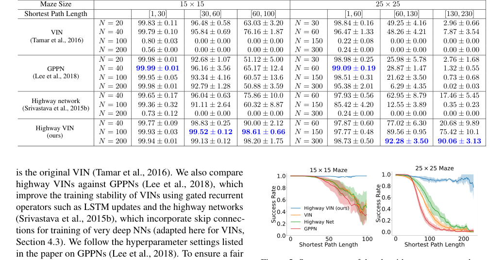Figure 5. Success rates of the algorithms are presented as a function of varying shortest path length. For each algorithm, the optimal result from a range of depths is selected. For a comprehensive view of the results across all depths, please see Fig. 9 in the Appendix

The paper also highlights the limitations of existing methods:
* The original VIN's performance drastically decreased with increasing depth, dropping to almost 0% SR for networks deeper than $N=150$. This is visually represented in Figure 1, which shows a 30-layer VIN's success rate falling below 10% for SPLs exceeding 120, and a 300-layer VIN exhibiting poor performance.
* While the Highway Network maintained performance at greater depths, it did not significantly improve long-term planning capabilities compared to its shallower counterparts.
* GPPN, though robust for short SPLs (achieving 99.09% SR for $25 \times 25$ maze with SPLs [1,30]), failed dramatically for longer paths, dropping below 3% for SPLs [130,230].

Further evidence of Highway VIN's effectiveness is provided by the learned feature maps (Figure 6). The feature maps of Highway VIN show larger learned values for states distant from the goal compared to VIN, indicating that Highway VIN develops a more effective and comprehensive value function for long-term planning.

The ablation studies provided crucial insights into the necessity of Highway VIN's novel components:
* Filter Gate: Figure 7 unequivocally shows that without the filter gate, Highway VIN's performance considerably decreases. This proves the filter gate's essential role in discarding "useless exploration paths" and ensuring convergence, directly validating its mathematical purpose.
* VE Modules: Figure 8 demonstrates a notable diminishment in performance when VE modules are absent, especially in the $25 \times 25$ maze. This confirms that the VE module's introduction of diverse latent actions is vital for facilitating information and gradient flow across spatial dimensions. Table 2 further quantifies this by showing that Highway VIN maintains significantly higher entropy of selected latent actions (e.g., 4.17 for $N=200$ in $15 \times 15$ maze) compared to VIN (0.00 for $N=200$), directly proving its ability to maintain diversity.

Finally, in 3D ViZDoom navigation (Table 3), Highway VIN again outperformed baselines, achieving a 96.98% SR for SPLs [60,100] compared to VIN's 69.37%, further solidifying its generalizability to more complex, visual environments. While Highway VIN did require more GPU memory (15.0G vs. 3.1G for VIN) and training time (9.0 hours vs. 7.5 hours for VIN) for 300 layers, this is a reasonable trade-off for the significant performance gains in long-term planning, especially when compared to GPPN's 103.0G memory usage.

Limitations & Future Directions

While Highway VIN presents a significant advancement in long-term planning for deep neural networks, the paper also implicitly and explicitly points to several limitations and opens avenues for future research.

One clear limitation, though a manageable one, is the increased computational cost for very deep Highway VINs. As shown in the computational complexity table, training a 300-layer Highway VIN requires more GPU memory (15.0G) and training time (9.0 hours) compared to a standard VIN (3.1G, 7.5 hours) or a Highway Network (3.3G, 7.7 hours). While this is still considerably more efficient than GPPN (103.0G), it suggests that scaling to even larger, more complex real-world problems might necessitate further optimization.

Another interesting observation, highlighted in Section B.2 and Figure 10, is that additional parallel VE modules ($N_p > 1$) can sometimes be detrimental to performance for very deep networks. For instance, at depth $N=300$, $N_p=1$ performs best, while at $N=100$, $N_p=3$ is optimal. This implies that the current mechanism for integrating multiple parallel VE modules might not be universally beneficial and could even hinder performance in certain deep configurations. This suggests a delicate balance or a need for more sophisticated strategies for combining these modules.

The paper also mentions that the embedded exploration rate $\epsilon=1$ (fully stochastic) is used during training, and while the filter gate prevents sub-optimal solutions, this fixed, maximal exploration might not be the most efficient or adaptive strategy for all scenarios. More dynamic or adaptive exploration mechanisms could potentially further improve learning efficiency or performance in environments with varying degrees of uncertainty or sparse rewards.

Looking forward, the authors explicitly propose two key directions in their conclusion:
1. Investigating the integration of multiple parallel VE modules with various types of embedded policies to improve performance. This directly addresses the limitation observed regarding $N_p > 1$ and suggests exploring more nuanced ways to leverage diverse planning horizons and policies.
2. Focusing on scaling up to larger tasks. The current experiments, while impressive, are primarily on maze navigation and a specific 3D environment. Extending Highway VIN to truly large-scale, high-dimensional, and unstructured real-world planning problems (e.g., complex robotics, autonomous driving in dynamic cities) would be a natural and crucial next step.

Beyond these, several discussion topics emerge for further development:
* Theoretical Robustness and Generalization: While the highway VI algorithm has convergence guarantees, a deeper theoretical analysis of the full differentiable Highway VIN architecture, especially concerning its stability and generalization properties in the presence of stochasticity and complex gate interactions, would be invaluable. This could provide stronger assurances for its deployment in safety-critical applications.
* Efficiency and Resource Optimization: Given the computational demands for very deep networks, future work could explore techniques like knowledge distillation to compress deep Highway VINs into shallower, more efficient models without significant performance loss. Additionally, investigating pruning strategies or hardware-aware optimizations could make these models more accessible for resource-constrained environments.
* Beyond Grid-World Planning: The current applications are grid-based or involve predicting grid-like maps. Exploring how Highway VIN can be adapted for continuous action spaces or graph-based planning problems where the state representation is not a simple grid would broaden its applicability. This might involve integrating different types of convolutional or graph neural network layers within the planning module.
* Interpretability and Explainability: While the learned feature maps offer some insight, further research into interpreting why Highway VIN makes certain planning decisions could be beneficial. Can we extract human-understandable planning heuristics or visualize the flow of "value" and "policy" information through the deep network to better understand its internal workings? This could help build trust and facilitate debugging in complex AI systems.
* Integration with Other RL Paradigms: How might Highway VIN integrate with other advanced reinforcement learning paradigms, such as model-based RL with learned world models or hierarchical RL? Could the planning module be used as a component within a larger, more sophisticated RL agent to tackle even more complex, multi-stage decision-making problems? This could lead to hybrid systems that combine the strengths of deep planning with other learning mechanisms.

Table 1. The success rates for each algorithm with various depths under 2D maze navigation tasks with different ranges of shortest path length. Please also refer to Appendix Table 4 for the results of all the other depths 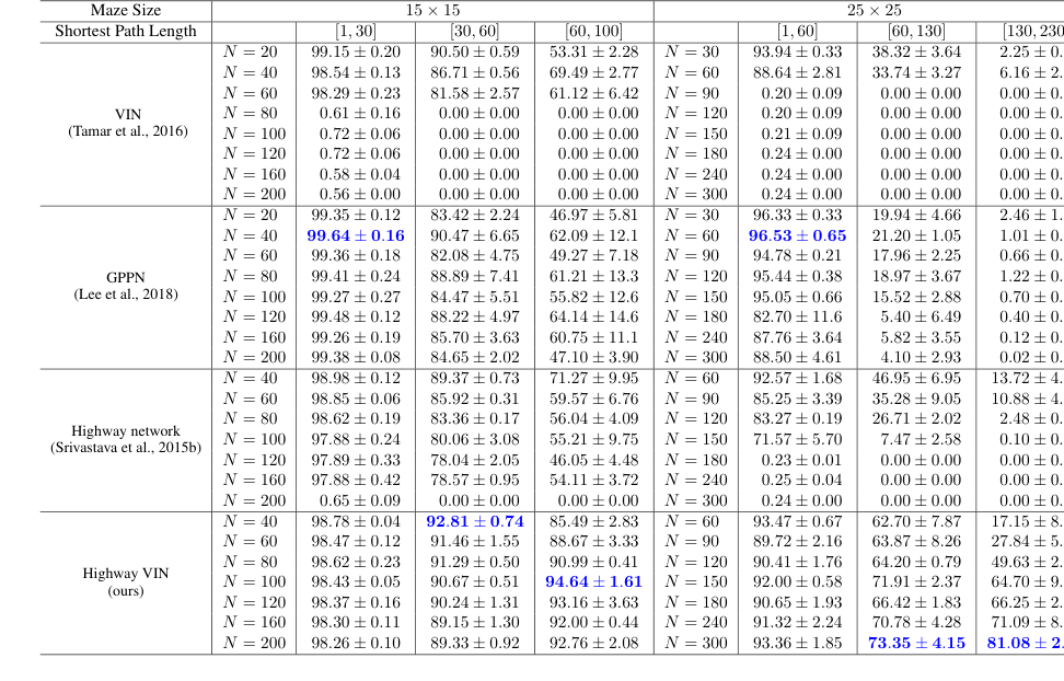Table 5. Optimality rates of each algorithm with various depths under 2D maze navigation tasks with different ranges of shortest path lengths. The optimality rate is defined by the ratio of tasks completed within the steps of the shortest path length to the total number of tasks 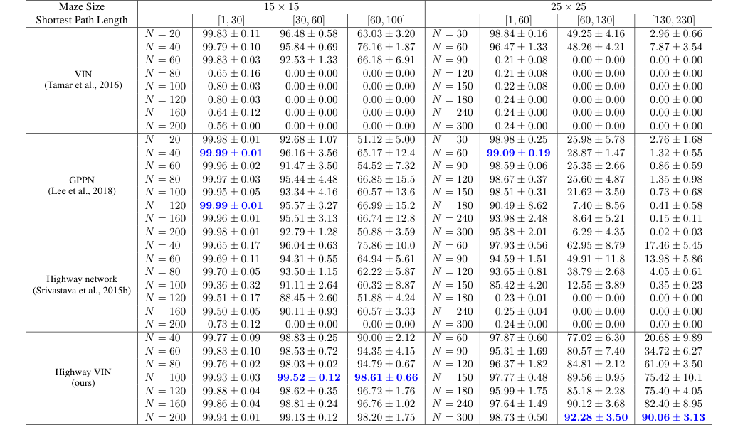Table 4. Success rates of each algorithm with various depths under 2D maze navigation tasks with different ranges of shortest path lengths