Generalization Bound and New Algorithm for Clean-Label Backdoor Attack

Background & Academic Lineage

The Origin & Academic Lineage

The problem addressed in this paper originates from the field of machine learning theory, specifically concerning the generalization capabilities of learning algorithms. Historically, the concept of a generalization bound has been a crucial theoretical tool for understanding how well a model trained on a finite dataset can perform on unseen data. Early work in this area, as referenced by Mohri et al. (2018), focused on metrics like VC-dimension and Rademacher complexity to quantify this generalization ability for standard learning tasks.

However, as machine learning models became more complex and applications diversified, new challenges emerged. One significant area of concern is data poisoning attacks, where malicious actors manipulate the training data to compromise the model's integrity. While generalization bounds for general data poisoning attacks have been explored (e.g., Wang et al., 2021; Hanneke et al., 2022), a specific and particularly insidious type of attack, the backdoor attack, presented a unique challenge.

The precise origin of this problem stems from the distinct characteristics of backdoor attacks. Unlike other data poisoning methods, a backdoor attack has a two-fold objective: first, to maintain high accuracy on normal, clean data, and second, to force the model to output a specific, targeted label when a particular "trigger" is present in the input. Crucially, this trigger is embedded in both the training and test sets. The existing generalization bounds were not designed to account for this dual objective or the non-i.i.d. (independent and identically distributed) nature of poisoned datasets, which is a fundamental assumption for classical generalization theory. The authors explicitly state that, to their knowledge, a generalization bound specifically for backdoor attacks had not been established, highlighting this as a significant gap in the academic literature that this paper aims to fill.

The fundamental limitation of previous approaches stemmed from their reliance on the i.i.d. condition, which is a cornerstone of classical generalization theory. Previous models and their associated bounds implicitly assumed that the training data was sampled independently and identically from the true data distribution. However, in the context of data poisoning, and especially backdoor attacks, the poisoned training dataset inherently violates this i.i.d. assumption. The introduction of triggers and targeted misclassifications means that the poisoned samples are no longer representative of the underlying clean data distribution in a straightforward manner. This violation rendered existing generalization bounds inapplicable, making it impossible to theoretically assess the generalizability of models trained under backdoor attack scenarios. This "pain point" forced the authors to develop new theoretical frameworks capable of handling the unique properties of clean-label backdoor attacks.

Intuitive Domain Terms

1. Generalization Bound:

   • Specialized Term: A mathematical upper limit on the difference between a model's performance on the training data and its performance on new, unseen data.
   • Intuitive Analogy: Imagine you're studying for a driving test. A "generalization bound" is like a guarantee that if you practice well on a specific set of roads (your training data), you'll perform within a certain margin of error on any new road you encounter during the actual test (unseen data). It tells you how reliably your learned skills will transfer to new situations.

2. Clean-Label Backdoor Attack:

   • Specialized Term: A type of data poisoning attack where a subtle, often imperceptible, trigger is added to a small subset of training data samples, but their original labels remain correct. The goal is for the trained model to classify any input containing this trigger as a specific target label, while still performing accurately on clean data.
   • Intuitive Analogy: Think of a dog show judge who is trained to identify different breeds. A "clean-label backdoor attack" is like someone secretly putting a tiny, unnoticeable red ribbon (the trigger) on a few dogs during training, but still telling the judge their correct breed. The judge learns to identify all breeds correctly. However, if any dog, even one never seen before, has that red ribbon, the judge is tricked into always calling it a "Poodle," regardless of its actual breed. The original labels of the poisoned training data were "clean" (correct), making the attack stealthy.

3. i.i.d. condition (Independent and Identically Distributed):

   • Specialized Term: A statistical assumption that all data samples are independent of each other and drawn from the same probability distribution.
   • Intuitive Analogy: This is like drawing cards from a perfectly shuffled deck. Each card you draw is "independent" of the previous one (it doesn't affect the next draw), and it comes from the "identical distribution" (the same deck). If someone secretly removes all the aces after your first few draws, the subsequent draws are no longer i.i.d. In machine learning, it means each piece of data is like a fresh, unbiased observation from the real world, and this assumption is crucial for many proofs to hold.

4. Rademacher Complexity:

   • Specialized Term: A measure of the "richness" or "capacity" of a hypothesis space (the set of all possible functions a model can learn). It quantifies how well a model can fit random noise.
   • Intuitive Analogy: Imagine a very flexible artist who can draw anything, even pure random scribbles. "Rademacher complexity" measures how good this artist is at perfectly replicating pure randomness. If the artist can perfectly draw any random scribble, they are extremely flexible (high complexity). In AI, it tells us how easily a model can memorize random noise, which is often a sign it's overfitting rather than learning true patterns.

5. Shortcut:

   • Specialized Term: A simple, easily learned feature that a model might exploit to make predictions, instead of learning the intended, more complex, and robust features.
   • Intuitive Analogy: If you're teaching a child to identify "cars," and all your training pictures of cars happen to have a specific brand logo in the corner, the child might learn to identify "that logo" as a "car" instead of the actual car features like wheels, windows, and shape. The logo is a "shortcut" feature that is easier to learn but doesn't generalize to real cars without that specific logo. The paper mentions that indiscriminate poison can be considered as such shortcuts.

Notation Table

Notation	Description

Problem Definition & Constraints

Core Problem Formulation & The Dilemma

The core problem addressed by this paper is the lack of theoretical understanding and generalization guarantees for clean-label backdoor attacks in deep learning.

Input/Current State:
The starting point is a standard machine learning setup where a neural network $F$ is trained on a clean training dataset $D_{tr} = \{(x_i, y_i)\}_{i=1}^N$. This dataset is assumed to be independently and identically distributed (i.i.d.) from an underlying data distribution $D_s$. The primary objective of such training is to minimize the population error $E_{(x,y) \sim D_s}[1(F(x) \neq y)]$, which measures the model's performance on unseen data. Existing generalization theory, including bounds based on VC-dimension, Rademacher complexity, or algorithmic stability, relies fundamentally on this i.i.d. assumption of the training data.

Desired Endpoint (Output/Goal State):
The paper aims to achieve a "clean-label backdoor attack" that is theoretically grounded. This involves creating a poisoned training set $D_p$ by subtly modifying a subset of the clean training data with a "trigger" $P(x)$, crucially without altering the original labels. A neural network $F$ trained on this $D_p$ must then satisfy a two-fold objective:
1. Maintain high accuracy on clean samples: The model should still perform well on unpoisoned, clean data, meaning its clean population error $E(F, D_s) = E_{(x,y) \sim D_s}[1(F(x) \neq y)]$ remains low.
2. Ensure targeted misclassification for triggered inputs: Any input $x$ that contains the trigger $P(x)$ (i.e., $x + P(x)$) should be classified by $F$ as a specific, pre-defined target label $l_p$. This is quantified by minimizing the poison population error $E_p(F, D_s) = E_{(x,y) \sim D_s}[1(F(x + P(x))) \neq l_p)]$.

The Dilemma & Missing Link:
The exact missing link is the establishment of robust generalization bounds for models trained under clean-label backdoor attack scenarios. The painful trade-off or dilemma that has trapped previous researchers is that backdoor attacks inherently violate the i.i.d. assumption of the training data. By introducing poisoned samples, the dataset $D_p$ is no longer i.i.d. sampled from $D_s$. This directly invalidates the foundational premise of classical generalization theory, making it impossible to directly apply existing bounds to guarantee the desired performance on both clean and triggered data.

Furthermore, for the poison generalization goal (Q2 in the paper), simply minimizing the empirical error on the poisoned training data $D_p$ does not automatically guarantee that any data with the trigger will be classified as the target label $l_p$. This is because if a clean sample $(x, y)$ with $y \neq l_p$ is not poisoned to $(x + P(x), l_p)$ in $D_p$, then minimizing empirical error on $D_p$ won't necessarily force the network to classify $x + P(x)$ as $l_p$. This highlights a subtle but critical gap between empirical performance on the poisoned training set and the desired generalization behavior for triggered inputs.

Constraints & Failure Modes

The problem of establishing generalization bounds for clean-label backdoor attacks is insanely difficult due to several harsh, realistic walls:

1. Non-i.i.d. Data Distribution: As highlighted, the most significant constraint is that the poisoned training dataset $D_p$ fundamentally does not satisfy the i.i.d. condition (Page 1, Abstract; Page 2, Q1 explanation). This is a direct consequence of the attack mechanism and renders standard generalization theories inapplicable. Developing new theoretical tools to handle this non-i.i.d. nature is a major hurdle.
2. Dual, Conflicting Objectives: The attack has two distinct goals: maintaining high accuracy on clean data and ensuring misclassification on triggered data. These objectives can be in tension. A model might overfit to the poisoned samples to achieve the backdoor, potentially degrading its performance on clean data, or vice versa. Balancing these two goals while providing theoretical guarantees is complex.
3. Clean-Label Stealthiness: The "clean-label" property means that the labels of poisoned samples are not changed. This makes the attack stealthier but also harder for the model to learn. The network must implicitly associate the trigger with the target label $l_p$ without explicit label guidance for the poisoned inputs, relying solely on the trigger's presence.
4. Specific Trigger Conditions for Poison Generalization: To ensure the poison generalization error is small, the trigger $P(x)$ cannot be arbitrary. Theorem 4.5 (Page 4) enumerates three critical conditions (c1, c2, c3) that $P(x)$ must satisfy:
   • (c1) Adversarial Noise: The trigger must act as adversarial noise for a network trained on clean data. This implies a need for specific perturbation properties.
   • (c2) Trigger Similarity: The trigger $P(x)$ must be similar across different input samples $x$. If triggers are highly varied, the model might struggle to generalize the backdoor behavior.
   • (c3) Shortcut Property: The trigger must function as a "shortcut" for a specially designed binary dataset. This is a non-trivial property to engineer and ensure, as it relates to how the trigger influences the model's decision boundary. Without these conditions, the attack's generalization to unseen triggered data is not guaranteed.
5. Computational and Attacker Resource Limits (Implicit): While not explicitly stated as "problem definition" constraints, the experimental setup (Section F.1, Page 32-33) reveals practical limitations that make the problem harder in real-world scenarios:
   • Limited Attacker Knowledge: The attacker is assumed to have limited knowledge of the victim network's structure and training process. This means triggers must be effective even when generated using smaller, proxy networks.
   • Limited Computing Power: The attacker is assumed to have limited computational resources, influencing the complexity of trigger generation algorithms.
   • Invisibility Constraints: Triggers are often constrained by $L_\infty$ norms (e.g., 16/255) to remain imperceptible (Page 6, 35). This physical constraint limits the magnitude of perturbations, making it more challenging to create effective and robust triggers.
6. Non-Differentiable Functions: The use of indicator functions $1(\cdot)$ for error calculation (e.g., $1(F(x) \neq y)$) introduces non-differentiability, which complicates direct optimization and theoretical analysis in some contexts. The paper uses cross-entropy loss (LCE) in Theorem 1.2 and 4.5, which is differentiable, but the ultimate goal is to bound the non-differentiable classification error.

Why This Approach

The Inevitability of the Choice

The authors' chosen approach, centered on deriving novel generalization bounds for clean-label backdoor attacks, was not merely one option among many, but rather the only viable solution to a previously unaddressed theoretical gap. The exact moment the authors realized traditional "SOTA" methods were insufficient is clearly articulated in the paper: "However, these generalization bounds are for clean training dataset and cannot be applied to poisoned training dataset, because poisoned datasets do not satisfy the i.i.d. condition, which is necessary for generalizibility" (Section 1, page 1).

This statement highlights a fundamental limitation of existing generalization theories, which typically assume data is independently and identically distributed (i.i.d.). Backdoor attacks, by their very nature, introduce carefully crafted perturbations into a subset of the training data, violating this crucial i.i.d. assumption. Therefore, standard generalization bounds, whether based on VC-dimension, Rademacher complexity, or specific to DNN architectures (e.g., CNNs, Transformers), are rendered inapplicable. The problem was not about finding a better model or algorithm within existing frameworks, but about establishing a new theoretical framework to understand the generalizability of attacks in a non-i.i.d. poisoned data setting. Furthermore, the unique two-fold objective of backdoor attacks—maintaining high accuracy on clean samples while ensuring targeted misclassification for triggered inputs—and the property that triggers exist in both training and test phases, necessitated a specialized theoretical treatment that existing methods simply did not provide.

Comparative Superiority

Beyond simple performance metrics like attack success rate (ASR) or clean accuracy, this method demonstrates qualitative superiority through its foundational theoretical grounding. Unlike many prior backdoor attacks that rely on empirical heuristics, the proposed approach is "based on generalization bounds and has certain theorectical guarantees" (Section 3, page 3). This means the attack is not just a black-box optimization but is designed with a deep understanding of the underlying conditions that enable its generalizability.

The method's structural advantage lies in its ability to identify and leverage specific mathematical conditions (c1, c2, c3 in Theorem 4.5) under which the poison generalization error can be controlled and minimized. This allows for a principled design of the poisoning trigger, combining adversarial noise and indiscriminate poison in a theoretically informed manner (Section 5, Remark 5.1). This is a significant qualitative leap over methods that might achieve high performance but lack a clear explanation of why they generalize or under what conditions they are guaranteed to work. The paper's approach provides a "more informed approach to using these methods" (Section 5, Remark 5.1), ensuring that the attack's effectiveness is rooted in a robust theoretical understanding rather than just empirical observation.

Alignment with Constraints

The chosen method perfectly aligns with the inherent constraints of clean-label backdoor attacks.

1. Clean-label nature: The entire theoretical framework and the proposed algorithm are specifically tailored for "clean-label backdoor attack[s], where poison triggers are added to a subset of the training set $D_{tr}$ without altering their labels" (Section 1, page 1). This is a core constraint that the paper directly addresses.
2. Two-fold attack goal: The problem defines two critical objectives: (1) maintaining high accuracy on clean samples, and (2) ensuring that any input with the trigger is classified as a targeted label $l_p$ (Section 3.2). The solution provides two distinct generalization bounds: Theorem 1.1 for the clean sample population error $E(F, D_s)$ and Theorem 1.2 for the poison population error $E_p(F, D_s)$, directly addressing both facets of the attack's goal.
3. Non-i.i.d. poisoned data: This is arguably the most challenging constraint. The paper explicitly states that "data in $D_p$ are no longer i.i.d. sampled from $D_s$, so the classical generalization bound cannot be used to obtain Theorem 1.1 directly" (Theorem 1.1, Q1). The authors overcome this by ingeniously identifying a subset of the poisoned training data that is i.i.d. sampled from the clean distribution (Proof idea for Theorem 4.1, page 4; Lemma A.3, page 14). This mathematical maneuver is a direct "marriage" between the problem's harsh data distribution requirement and the solution's unique theoretical properties.
4. Trigger presence in both training and test phases: The generalization bounds are formulated to account for triggers in both phases. The empirical error on the poisoned training set $D_p$ is used to bound population errors, inherently considering the trigger's role during training. The poison generalization error $E_p(F, D_s)$ directly evaluates the attack's success on triggered test data.
5. Stealthiness/Invisibility: While primarily an experimental constraint, the proposed Algorithm 1 incorporates a "poison budget $\eta$" (Algorithm 1, Input) which can be set to enforce $L_\infty$ norm bounds (e.g., 16/255), ensuring that the generated triggers remain imperceptible, aligning with practical requirements for stealthy attacks.

Rejection of Alternatives

The paper implicitly and explicitly rejects several alternative approaches, primarily by highlighting the unique challenges of clean-label backdoor attacks that existing methods fail to address.

Firstly, the most direct rejection is of "classical generalization bounds" (Section 1, page 1). These bounds, whether based on VC-dimension, Rademacher complexity, or specific to deep neural networks, are deemed insufficient because they assume i.i.d. data. Poisoned datasets, by definition, violate this assumption, making these traditional theoretical tools inapplicable. The authors' work fills this fundamental gap, implying that simply adapting or applying existing generalization theories would have failed.

Secondly, the paper differentiates its work from other existing generalization bounds for data poisoning attacks (e.g., Wang et al., 2021; Hanneke et al., 2022). It states that "Our result is different from these works and cannot be derived from them" (Section 2, page 3). The reasoning is that these prior works do not account for the specific properties of backdoor attacks, such as the trigger being present in both training and inference phases, and the two-fold goal of maintaining clean accuracy while achieving targeted misclassification. This implies that these more general poisoning generalization bounds are not granular enough for the nuances of clean-label backdoor attacks.

Finally, regarding the attack generation methods themselves, the paper implicitly rejects purely empirical or heuristic-based approaches by emphasizing that "Most existing backdoor attacks are mainly based on empirical heuristics, while our attack is based on generalization bounds and has certain theoretical guarantees" (Section 3, page 3). When comparing with other clean-label attacks (Section 6.3, Table 4), the authors note that many alternatives require "additional steps," "pre-existing patches," "fitting images," "magnifying triggers," or "large generative models" (Section 6.3). For instance, "Invisible Poison" and "Image-specific" attacks rely on large generative models for optimal performance, which the proposed method avoids. The theoretical guidance of the new algorithm allows for a more efficient and principled trigger design, circumventing the need for these often complex, resource-intensive, or ad-hoc components of other attacks. This makes the proposed method qualitatively superior due to its robust theoretical foundation, leading to better accuracy and attack success rates without such overheads.

Figure 4. When trigger is a patch without norm limitation, it is not invisible. This figure is from (Souri et al., 2022)

Mathematical & Logical Mechanism

The Master Equation

The paper's core contribution lies in establishing generalization bounds for clean-label backdoor attacks, addressing two primary objectives: maintaining high accuracy on clean samples and ensuring successful classification of triggered data to a target label. These objectives are mathematically captured by two master equations, derived as Theorem 4.1 and Theorem 4.5, respectively.

The clean generalization error bound (Theorem 4.1) is given by:
$$ E(F,D_s) \leq \frac{4-2\alpha}{1-\alpha} E(F,D_p) + O\left(\frac{mW^2D^2}{N} \ln(2/\delta) + \sqrt{\frac{\alpha}{N(1-\alpha)}}\right) $$

The poison generalization error bound (Theorem 4.5) is given by:
$$ E_p(F,D_s) \leq \lambda O\left(\left(E_{(x,y)\in D_p} [L_{CE}(F(x), y)] + \text{Rad}_{D_p}^{D_s}(H_{W,D,1})\right) + \sqrt{\frac{\ln(1/\delta)}{N\alpha}} + \epsilon + \tau + \lambda\right) $$

Term-by-Term Autopsy

Let's dissect each component of these equations to understand their mathematical definition, physical/logical role, and the author's rationale for their inclusion and operation.

Equation 1: Clean Generalization Error Bound

• $E(F,D_s)$

  • Mathematical Definition: This is the population error of the neural network $F$ on the true, underlying data distribution $D_s$. It is formally defined as $E_{(x,y)\sim D_s} [1(F(x) \neq y)]$, where $1(\cdot)$ is the indicator function that returns 1 if its argument is true, and 0 otherwise.
  • Physical/Logical Role: This term represents the model's true error rate on clean, unpoisoned data that it has never seen before. In the context of a backdoor attack, a primary goal is to keep this value small, ensuring the model remains useful for its intended, legitimate tasks.
  • Why used: It's the ultimate metric for evaluating the model's performance on clean data, which is a key requirement for a stealthy backdoor attack.

• $\leq$

  • Mathematical Definition: "Less than or equal to."
  • Physical/Logical Role: This symbol signifies that the expression on the right-hand side provides an upper bound for the true population error on the left. This is the essence of a generalization bound.
  • Why used: Since the true data distribution $D_s$ is unknown, $E(F,D_s)$ cannot be directly computed. Generalization theory provides probabilistic upper bounds based on observable quantities.

• $\frac{4-2\alpha}{1-\alpha}$

  • Mathematical Definition: A scalar coefficient that depends on $\alpha$, the poisoning ratio (percentage of samples labeled $l_p$ in $D_{tr}$ that are poisoned).
  • Physical/Logical Role: This coefficient scales the empirical error observed on the poisoned training data. It reflects how the proportion of poisoned samples impacts the tightness of the generalization bound. As $\alpha$ increases, this coefficient generally grows, indicating a potentially looser bound or a greater divergence between empirical and population error.
  • Why used: The paper highlights that poisoned datasets ($D_p$) do not satisfy the i.i.d. (independent and identically distributed) condition, which is a prerequisite for classical generalization bounds. This coefficient likely emerges from the specific mathematical techniques employed to adapt generalization theory to this non-i.i.d. setting.

• $E(F,D_p)$

  • Mathematical Definition: This is the empirical error of the network $F$ on the poisoned training dataset $D_p$. It is defined as $E_{(x,y)\in D_p} [1(F(x) \neq y)]$.
  • Physical/Logical Role: This represents the error rate of the model as measured directly on the finite training data, which includes both clean and poisoned samples. This is the quantity that the learning algorithm actively tries to minimize during training.
  • Why used: It's the observable, measurable error during the training process. Generalization bounds aim to connect this empirical performance to the unobservable true performance.

• $O(\cdot)$

  • Mathematical Definition: Big O notation, indicating an asymptotic upper bound on the growth rate of a function. It means the terms inside grow no faster than the specified function.
  • Physical/Logical Role: This notation groups together terms that constitute the "generalization gap." These terms typically decrease as the size of the training dataset $N$ increases, implying that with more data, the empirical error becomes a more reliable estimate of the population error.
  • Why used: It simplifies the expression by abstracting away less significant constants and focusing on the dominant factors that determine how quickly the generalization gap closes.

• $\frac{mW^2D^2}{N} \ln(2/\delta)$

  • Mathematical Definition: A term related to model complexity, data size, and confidence.
    • $m$: The number of classes in the label set.
    • $W$: The width of the neural network (e.g., maximum number of neurons in a layer).
    • $D$: The depth of the neural network (number of layers).
    • $N$: The total number of samples in the clean training set $D_{tr}$.
    • $\ln(2/\delta)$: The natural logarithm of $2/\delta$, where $\delta$ is a small probability (e.g., 0.05) that the derived bound might not hold (i.e., the bound holds with probability $1-\delta$).
  • Physical/Logical Role: This term quantifies the capacity of the neural network model. A more complex model (larger $W$ or $D$) has a greater ability to fit the training data, including noise, which can lead to a larger generalization gap (overfitting). Conversely, a larger training set size $N$ helps reduce this gap. The $\ln(2/\delta)$ factor accounts for the probabilistic nature of the bound. This term is characteristic of bounds derived using concepts like Rademacher complexity or VC-dimension.
  • Why used: It's a standard component in generalization bounds for deep learning models, reflecting the trade-off between model expressiveness and the amount of available data.

• $\sqrt{\frac{\alpha}{N(1-\alpha)}}$

  • Mathematical Definition: A square root term involving the poisoning ratio $\alpha$ and the training set size $N$.
  • Physical/Logical Role: This term specifically captures the statistical uncertainty introduced by the poisoning process. As the poisoning ratio $\alpha$ increases, this term generally increases, suggesting a larger generalization gap due to the increased perturbation of the data distribution. Conversely, a larger $N$ reduces this term, indicating that more data can help mitigate the adverse effects of poisoning. The $(1-\alpha)$ in the denominator implies that if almost all samples are poisoned ($\alpha \to 1$), the bound becomes very loose.
  • Why used: This term directly addresses the unique challenge of generalization in the presence of data poisoning, quantifying the statistical impact of the non-i.i.d. nature of the poisoned dataset.

Equation 2: Poison Generalization Error Bound

• $E_p(F,D_s)$

  • Mathematical Definition: This is the poison population error of the network $F$ on the true data distribution $D_s$. It is formally defined as $E_{(x,y)\sim D_s} [1(F(x + P(x))) \neq l_p)]$, where $P(x)$ is the trigger applied to input $x$, and $l_p$ is the designated target label for triggered inputs.
  • Physical/Logical Role: This term measures the true failure rate of the backdoor attack on unseen, triggered data. The goal of the attack is to make this value as small as possible, ensuring that any input with the trigger is consistently classified as $l_p$.
  • Why used: It's the critical metric for evaluating the success rate and effectiveness of the backdoor attack itself.

• $\leq$

  • Mathematical Definition: "Less than or equal to."
  • Physical/Logical Role: Similar to Equation 1, this indicates that the right-hand side provides an upper bound for the poison population error.
  • Why used: It establishes a theoretical guarantee for the backdoor attack's effectiveness, bounding its true error rate.

• $\lambda$

  • Mathematical Definition: A scaling factor derived from condition (c2) in Theorem 4.5, which states $P_{(x,y)\sim D_s}(P(x) \in A|y \neq l_p) \leq \lambda P_{(x,y)\sim D_s}(P(x) \in A|y = l_p)$ for any set $A$.
  • Physical/Logical Role: This parameter quantifies the "similarity" or "consistency" of the trigger $P(x)$ across different clean samples $x$. If $P(x)$ is highly similar for various inputs, $\lambda$ approaches 1. A smaller $\lambda$ (closer to 1) is desirable for a tighter bound, implying that the trigger acts as a general, consistent pattern that the model can easily learn.
  • Why used: It's a crucial condition for designing effective triggers, ensuring that the backdoor is not tied to specific input characteristics but rather to the trigger itself, making it generalizable.

• $O(\cdot)$

  • Mathematical Definition: Big O notation, similar to Equation 1.
  • Physical/Logical Role: Groups terms contributing to the generalization gap for the poison population error.
  • Why used: Simplifies the bound by focusing on dominant factors.

• $E_{(x,y)\in D_p} [L_{CE}(F(x), y)]$

  • Mathematical Definition: This is the empirical cross-entropy loss of the network $F$ on the poisoned training dataset $D_p$. $L_{CE}$ denotes the cross-entropy loss function.
  • Physical/Logical Role: This term represents the empirical risk (loss) that the model minimizes during training on the poisoned dataset. Unlike the 0-1 error, cross-entropy loss provides a continuous measure of how confident the model is in its predictions, encouraging it to output the target label $l_p$ with high probability for triggered inputs.
  • Why used: Cross-entropy loss is a standard and more informative loss function for classification tasks, especially when high confidence in specific predictions is desired, as is the case for backdoor attacks.

• $\text{Rad}_{D_p}^{D_s}(H_{W,D,1})$

  • Mathematical Definition: The Rademacher complexity of the hypothesis space $H_{W,D,1}$ under a distribution that bridges $D_p$ and $D_s$. $H_{W,D,1}$ is the set of functions $h_F(x,y) = F_y(x)$ for neural networks $F$ with width $W$ and depth $D$. The notation suggests it's a Rademacher complexity calculated from samples in $D_p$ but intended to generalize to $D_s$.
  • Physical/Logical Role: This term quantifies the "learnability" or "flexibility" of the model class in the context of the poisoned data. A higher Rademacher complexity indicates a model that can fit more complex patterns, potentially leading to overfitting if not properly controlled. It measures the model's ability to fit random labels, which is a proxy for its capacity to overfit.
  • Why used: Rademacher complexity is a fundamental tool in statistical learning theory for bounding generalization error, especially for complex function classes like neural networks.

• $\sqrt{\frac{\ln(1/\delta)}{N\alpha}}$

  • Mathematical Definition: A square root term involving the confidence parameter $\delta$, the training set size $N$, and the poisoning ratio $\alpha$.
  • Physical/Logical Role: This term represents a statistical concentration component. As $N$ increases, this term decreases, leading to a tighter bound. A smaller $\alpha$ (fewer poisoned samples) makes this term larger, indicating that it's harder to statistically generalize about the poison's effect with very few samples.
  • Why used: This is a common term in concentration inequalities, reflecting the sample complexity required to achieve a certain confidence level for the bound.

• $\epsilon$

  • Mathematical Definition: A small positive value from condition (c1) in Theorem 4.5: $E_{(x,y)\sim D_p^{l_p}} [G_y(x + P(x))] \leq \epsilon$. Here, $G_y(x)$ is the probability that a clean-trained network $G$ classifies $x$ as $y$.
  • Physical/Logical Role: This term quantifies how "adversarial" the trigger $P(x)$ is. If $P(x)$ effectively causes a clean-trained network $G$ to misclassify $x+P(x)$, then $\epsilon$ will be small. A smaller $\epsilon$ is desired for a tighter bound, meaning the trigger should be an effective adversarial perturbation.
  • Why used: It's a condition on the trigger design, ensuring that the trigger can effectively "fool" a clean model, which is a characteristic of many backdoor attacks.

• $\tau$

  • Mathematical Definition: A small positive value from condition (c3) in Theorem 4.5: $E_{x\sim D_s} [|(F-G)_{l_p}(P(x)) - (F-G)_{l_p}(x+P(x))|] \leq \tau$. This measures the similarity of the "backdoor part" of the network's output for $P(x)$ and $x+P(x)$.
  • Physical/Logical Role: This term quantifies how "shortcut-like" the trigger $P(x)$ is. If the trigger acts as a shortcut, the network's response to $P(x)$ alone should be similar to its response to $x+P(x)$, leading to a small $\tau$. A smaller $\tau$ is desired for a tighter bound, meaning the trigger creates a strong, direct path to the target label.
  • Why used: It's a condition on the trigger design, encouraging the model to learn the trigger as a simple, direct feature (a "shortcut") rather than a complex interaction with the original input.

• Why addition instead of multiplication, or integral instead of summation?
  The equations are structured as sums because they aggregate different sources of error and factors contributing to the generalization gap. Each term represents a distinct aspect: the empirical error (what's observed), model complexity, statistical variance, and specific properties of the trigger. These factors contribute additively to the overall upper bound on the population error. For instance, both model complexity and statistical uncertainty independently increase the potential for the empirical error to deviate from the true population error.

  The notation $E_{(x,y)\sim D_s}$ implies an expectation over a continuous probability distribution $D_s$, which is mathematically represented by an integral. In contrast, $E_{(x,y)\in D_p}$ denotes an empirical average over a finite, discrete dataset $D_p$, which is calculated as a summation. The authors use the appropriate mathematical operator (integral or summation) implicitly through their expectation notation, depending on whether they refer to a continuous population or a discrete sample.

Step-by-Step Flow

Let's trace the journey of a single abstract data point, $(x_0, y_0)$, from the true data distribution $D_s$, through the conceptual mechanism described by these generalization bounds.

1. Origin of Data Point: Our journey begins with an abstract, clean data point $(x_0, y_0)$, where $x_0$ is an input (e.g., an image) and $y_0$ is its true label. This point is a representative sample from the infinite, unobservable true data distribution $D_s$.

2. Hypothetical Poisoning for Attack Evaluation: If we are evaluating the poison population error $E_p(F,D_s)$, this clean input $x_0$ is conceptually modified by adding a pre-designed trigger $P(x_0)$. The resulting input becomes $x_0 + P(x_0)$, and its intended label for the backdoor attack is $l_p$, regardless of $y_0$. This transformed pair $(x_0 + P(x_0), l_p)$ represents what the attacker wants the model to classify correctly. For evaluating clean generalization error $E(F,D_s)$, the data point remains $(x_0, y_0)$.

3. Model Inference (The "Black Box" Network $F$): The (hypothetically) trained neural network $F$ receives this input.

   • Feature Transformation: The input (either $x_0$ or $x_0 + P(x_0)$) passes through the network's layers. Each layer, composed of operations like convolutions, non-linear activations (e.g., ReLU), and pooling, progressively transforms the raw input into more abstract and discriminative feature representations.
   • Output Generation: The final layer of the network, typically a Softmax layer, converts these features into a probability distribution over all possible output classes. $F(z)$ is this vector of probabilities, where $F_y(z)$ is the probability assigned to label $y$ for input $z$.
   • Classification Decision: The network's final classification $\text{argmax}_y F_y(z)$ is the label with the highest predicted probability.

4. Error/Loss Calculation (Population Level):

   • Clean Error: For clean generalization, the network's output $F(x_0)$ is compared against the true label $y_0$. If the predicted label $\text{argmax}_y F_y(x_0)$ does not match $y_0$, an error is registered. This process is conceptually repeated and averaged over all possible $(x,y) \sim D_s$ to yield $E(F,D_s)$.
   • Poison Error: For poison generalization, the network's output $F(x_0 + P(x_0))$ is compared against the target label $l_p$. If $\text{argmax}_y F_y(x_0 + P(x_0))$ does not match $l_p$, an error is registered. This is averaged over all possible $(x,y) \sim D_s$ to obtain $E_p(F,D_s)$.

5. Empirical Counterpart (Training Data $D_p$): During the actual training phase, the model $F$ is exposed to a finite, observable, and poisoned training dataset $D_p$.

   • Sample Selection: A specific sample $(x_i, y_i)$ is drawn from $D_p$. This sample could be an original clean sample from $D_{tr}$ or a poisoned sample $(x_j + P(x_j), l_p)$ that was created by perturbing a clean sample $(x_j, l_p)$ from $D_{tr}$.
   • Empirical Loss/Error: The network $F$ processes $x_i$.
     • For the clean generalization bound, the empirical error $E(F,D_p)$ is calculated by comparing $F(x_i)$ to $y_i$ using the indicator function.
     • For the poison generalization bound, the empirical cross-entropy loss $L_{CE}(F(x_i), y_i)$ is computed. This measures how well $F$ predicts $y_i$ for input $x_i$.
   • Averaging: These individual errors or losses are then averaged over all samples in the finite dataset $D_p$ to yield $E(F,D_p)$ or $E_{(x,y)\in D_p} [L_{CE}(F(x), y)]$.

6. Bridging the Generalization Gap: The mathematical engine then connects these observable empirical errors/losses on $D_p$ to the unobservable true population errors on $D_s$. The additional terms in the bounds (Rademacher complexity, $\sqrt{\frac{\ln(1/\delta)}{N\alpha}}$, $\epsilon$, $\tau$, $\lambda$) act as "correction factors" or "penalty terms." They quantify:

   • Model Capacity: How prone the network $F$ is to overfitting (Rademacher complexity).
   • Data Scarcity: The statistical uncertainty due to having a finite training set ($N$).
   • Poisoning Impact: The specific statistical biases introduced by the poisoning ratio ($\alpha$).
   • Trigger Quality: How well the crafted trigger $P(x)$ fulfills the desired properties of being adversarial ($\epsilon$), consistent ($\lambda$), and a shortcut ($\tau$).

This entire process makes the abstract math feel like a moving mechanical assembly line: raw data enters, gets processed by a machine (the network), and its performance is measured. The generalization bounds then provide a theoretical "quality control" report, predicting the machine's performance on future, unseen data based on its observed performance and inherent design characteristics.

Optimization Dynamics

The generalization bounds themselves are not direct optimization objectives for the victim model $F$. Instead, they provide theoretical guarantees and conditions under which a backdoor attack will generalize effectively. The "optimization dynamics" in this context refer to how the trigger $P(x)$ is designed to satisfy these conditions, and how the victim model $F$ is trained to achieve the desired backdoor behavior while adhering to these bounds.

The paper's proposed algorithm (Algorithm 1) for creating the poisoning trigger $P(x)$ is where the primary optimization dynamics for the attack itself occur:

1. Crafting Adversarial Disturbance (Satisfying Condition c1/t1 for small $\epsilon$):

   • Mechanism: A network $F_1$ is trained on a clean dataset $T$. For each clean sample $x$, an adversarial perturbation $x_{adv}$ is generated using Projected Gradient Descent (PGD). PGD is an iterative optimization process that finds a small perturbation $\epsilon$ (within an $L_\infty$ budget $\eta$) that maximizes the loss of $F_1$ for the original label $y$.
   • Gradients & Loss Landscape: This involves computing the gradients of the loss function $L(F_1(x+\epsilon), y)$ with respect to $\epsilon$. The optimization iteratively updates $\epsilon$ by taking steps in the direction of the gradient (gradient ascent) to increase the loss, then projecting $\epsilon$ back into the allowed perturbation space. This process shapes the "adversarial" component of the trigger, aiming to make $\epsilon$ (which contributes to $P(x)$) an effective adversarial example, thus ensuring $\epsilon$ in the bound is small.

2. Crafting Shortcut Disturbance (Satisfying Condition c3/t3 for small $\tau$):

   • Mechanism: A separate, simpler two-layer network $F_2$ is trained on a specially constructed dataset $T_1$. This dataset includes clean samples and samples perturbed by $x_{adv}$ (from the previous step), but with a specific label (0). The goal is to find a "shortcut" perturbation $x_{scut}$ using a min-min method. This method aims to make the poisoned dataset linearly separable by $F_2$.
   • Loss Landscape & State Updates: The min-min method typically involves an inner optimization loop (finding the best $x_{scut}$ for a given $F_2$) and an outer optimization loop (training $F_2$). The loss landscape for $F_2$ is shaped to encourage it to learn simple, linear-separable features from the poisoned data. This effectively creates a "shortcut" that maps the trigger to the target label. The iterative updates of $F_2$'s parameters and $x_{scut}$ aim to minimize $\tau$, ensuring the trigger acts as a strong shortcut feature.

3. Combining Disturbances (Satisfying Condition c2/t2 for $\lambda$ close to 1):

   • Mechanism: The final trigger $P(x)$ is constructed by combining $x_{adv}$ and $x_{scut}$ using a binary mask $U$: $P(x) = U \odot x_{adv} + (1-U) \odot x_{scut}$. The mask $U$ is designed (e.g., a specific region like the upper-left corner is 0, and the rest is 1) to ensure that the shortcut component $(1-U) \odot x_{scut}$ is similar across different inputs $x$.
   • Behavior of Gradients/State Updates: While there isn't a direct gradient-based optimization for $\lambda$ itself, the design choice of the mask $U$ and the properties of the min-min method (which tends to produce similar shortcuts for different inputs) implicitly guide the trigger generation towards satisfying condition (c2). This ensures that the trigger is a consistent pattern, making $\lambda$ in the bound approach 1. Some poisons obtained using Algorithm 1 are shown in Figure 1.

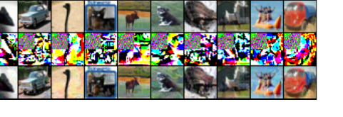Figure 1. From top row to bottom row are respectively the clean images, normalized triggers (original trigger has L∞norm bound 16/255), poison images. Due to the selection of U, the upper left corners of the poison images are similar, while the other parts are used to generate adversaries

1. Victim Model Training and Convergence:
   • Mechanism: Once the triggers $P(x)$ are generated, they are applied to a subset of the original clean training data $D_{tr}$ to form the poisoned training set $D_p$. The victim network $F$ is then trained on $D_p$ using standard optimization algorithms like Stochastic Gradient Descent (SGD) with a cross-entropy loss function.
   • Loss Landscape & Convergence: The presence of poisoned samples in $D_p$ modifies the loss landscape for the victim model $F$. The model learns to minimize the empirical loss on $D_p$, which means it must learn both the clean classification task for unpoisoned samples and the backdoor task for triggered samples. The generalization bounds then predict the behavior of this converged model $F$. If the trigger $P(x)$ was successfully crafted to meet the conditions (small $\epsilon, \tau$, $\lambda$ close to 1), the bounds suggest that the victim model, upon convergence, will exhibit high clean accuracy and a high attack success rate. The iterative updates of $F$'s parameters via SGD drive it towards a local minimum in this complex, multi-objective loss landscape.

In essence, the optimization dynamics are a two-stage process: first, a targeted, gradient-driven optimization to craft the trigger $P(x)$ to possess specific properties (adversarial, shortcut, consistent) that are mathematically linked to the generalization bounds; and second, the standard training of the victim network on the resulting poisoned dataset, where the bounds then predict the generalization performance of the final model. The bounds provide the theoretical framework for why these trigger design principles lead to an effective and generalizable backdoor attack.

Results, Limitations & Conclusion

Experimental Design & Baselines

To rigorously validate their theoretical claims and the efficacy of the proposed clean-label backdoor attack, the authors conducted extensive experiments across various benchmark datasets and victim network architectures. The experimental setup was meticulously designed to simulate practical attack scenarios, where the attacker has limited knowledge and control over the victim's training process.

Datasets and Victim Models: The attack was evaluated on widely-used image classification datasets: CIFAR10, CIFAR100, SVHN, and TinyImageNet. For victim models, popular deep neural networks like VGG16, ResNet18, and WRN34-10 were employed.

Attack Mechanism and Trigger Generation: The core of the proposed attack involves a novel trigger generation method (Algorithm 1) that combines adversarial noise and indiscriminate poison. This process itself utilizes smaller, independent networks (F1 for adversarial noise, F2 for shortcut disturbance) to avoid assumptions about the victim network's structure or computational power. For instance, F1 was trained using PGD-10 adversarial training with L-infinity norm budgets (e.g., 8/255 or 4/255), while F2, a two-layer network, was trained using the Min-Min method to create shortcuts. The poisoning process involved randomly selecting a subset of training samples (e.g., 1% or 0.8% of training images) with a specific target label $l_p$ (typically set to 0) and adding the generated trigger to them without altering their original labels.

Evaluation Metrics and Baselines: The effectiveness of the attack was primarily measured by:
1. Clean Model Accuracy: The accuracy of the poisoned model on clean test samples.
2. Poisoned Model Accuracy: The accuracy of the poisoned model on poisoned test samples.
3. Attack Success Rate (ASR): The rate at which samples containing the trigger are misclassified as the target label $l_p$.
4. Clean Model $l_p$ Accuracy: The accuracy of clean samples belonging to the target class $l_p$.

The proposed method was benchmarked against seven prominent clean-label backdoor attacks: Clean Label, Hidden Trigger, Reflection, Invisible Poison, Image-specific, Narcissus, and Sleeper Agent. For fair comparison, all attacks were constrained by an L-infinity norm trigger budget (e.g., 16/255) and a fixed poison budget (e.g., 1% of training images).

Defense Mechanisms: To assess the robustness of the attack, it was tested against six common backdoor defenses: Adversarial Training (AT), Data Augmentation, Scale-up, Differentially Private SGD (DPSGD), Frequency Filter, and Fine-Tuning.

Theoretical Verification: Beyond empirical performance, the authors conducted ablation studies to verify their mathematical claims, specifically Theorems 4.1 and 4.5. This involved analyzing how different components of the trigger (adversarial noise, shortcut noise) influenced the conditions (c1), (c2), (c3) of Theorem 4.5, using metrics like $V_{adv}$ (validation loss on poisoned data for condition (c1)) and $V_{sc}$ (binary classification loss for condition (c3)). They also investigated the impact of poison rate on overall accuracy to support Theorem 4.1.

What the Evidence Proves

The experimental evidence provides compelling support for the effectiveness and theoretical underpinnings of the proposed clean-label backdoor attack.

Definitive Evidence of Core Mechanism:
The core mechanism, which combines adversarial noise and indiscriminate poison to create triggers that satisfy the conditions of Theorem 4.5, was ruthlessly proven effective. The attack consistently achieved high Attack Success Rates (ASR) while maintaining high accuracy on clean samples, which are the two primary goals of a clean-label backdoor attack. For instance, on CIFAR-10 with ResNet18 and a 1% poison budget (L-infinity norm 16/255), the proposed method achieved an ASR of 93%, with clean model accuracy at 93% and poisoned model accuracy at 91% (Table 1). This demonstrates that the victim model learned the trigger to misclassify inputs to the target label $l_p$ while still performing well on legitimate, clean data.

The "victims" (baseline models) were decisively defeated. Under an L-infinity norm budget of 16/255, our attack achieved a 93% ASR on CIFAR-10, significantly outperforming all other compared methods, which ranged from 23% (Clean-Label) to 75% (Hidden-Trigger) (Table 4). This undeniable evidence highlights that the specific combination of adversarial noise and shortcut properties in the trigger, guided by the theoretical bounds, is superior in implanting effective backdoors. The attack's efficacy remained high even with very small poison budgets (e.g., 86% ASR for 0.6% poison budget on CIFAR-10 with ResNet18, Table 2), further proving its potency.

The attack's performance was consistent across various datasets (CIFAR10, CIFAR100, SVHN, TinyImageNet) and different target labels (0-9), as shown in Tables 3 and Figure 3. This indicates a generalizable attack strategy rather than one specific to a particular dataset or target class. The training process monitoring (Figure 2) further confirmed that the clean and poisoned model accuracies remained close, and the ASR quickly stabilized at a high level, indicating robust learning of the backdoor.

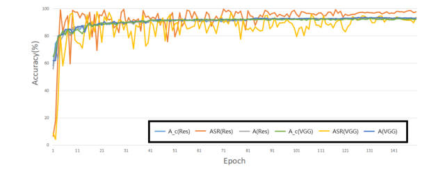Figure 2. Attack performance during the training process on CIFAR10 with ResNet18 and VGG16. This figure shows the trend of the poison model accuracy (A), attack success rate (ASR) and clean model accuracy (Ac)

Verification of Theoretical Claims:
The ablation studies specifically designed to verify Theorem 4.5 provided crucial insights. By comparing different poison types (Random Noise, Universal Adversarial, Adversarial, Shortcut, and Ours) and evaluating their impact on $V_{adv}$ (related to condition c1) and $V_{sc}$ (related to condition c3), the authors showed that individual components often excel in one condition but fail in another. For example, adversarial perturbations alone ($Adv$) resulted in a high $V_{adv}$ (meaning condition c1 was not well satisfied), while shortcut noise ($SCut$) alone resulted in a high $V_{sc}$ (meaning condition c3 was not well satisfied). However, the proposed "Ours" method, which combines both, achieved a balanced outcome with good $V_{adv}$ and very low $V_{sc}$, leading to a significantly higher ASR (93% for Ours vs. 22% for Adv and 30% for SCut under 16/255 budget, Table 6). This directly validates that satisfying the conditions of Theorem 4.5 through a combined trigger mechanism leads to superior attack performance.

Regarding Theorem 4.1, the experiments showed that while a higher poison rate generally leads to a greater impact on clean accuracy, the decline is not significant (e.g., only a 4% decrease for over 3,000 poisoned samples, Table 14). This supports the theoretical insight that the poisoning ratio affects generalizability, but also that with controlled poison budgets, the impact on clean sample accuracy can be minimized. Furthermore, the victim network was shown to learn the trigger features effectively (Table 12), yet it still prioritized original image features, necessitating a sufficient scale of poison for the backdoor to be effective.

Limitations & Future Directions

While the proposed clean-label backdoor attack demonstrates remarkable effectiveness and is grounded in solid theoretical generalization bounds, the paper acknowledges several limitations and opens avenues for future research.

Current Limitations:
One significant limitation lies in the complexity of the conditions outlined in Theorem 4.5. The authors themselves state that these conditions are "quite complicated," and deriving simpler, more intuitive conditions for the poisoned population error bound would be highly desirable. This complexity might hinder broader understanding and application of the theoretical framework.

Another theoretical gap is that the current generalization bounds do not explicitly incorporate the training process. Algorithmic-dependent generalization bounds, particularly those based on stability analysis (e.g., Hardt et al., 2016), warrant further investigation in the context of backdoor attacks. Such analysis could provide a more fine-grained understanding of how the training dynamics influence the attack's success and generalizability.

From a practical standpoint, the paper notes that the generated triggers exhibit limited transferability across different datasets. A trigger created for CIFAR-10, for instance, cannot be directly applied to CIFAR-100 (Appendix F.5). This restricts the attack's versatility and requires re-generating triggers for each new dataset, which can be computationally intensive.

Furthermore, the attack, while highly effective against baselines, appears "somewhat fragile under defense" (Section 6.4). Although the authors propose "enhanced attacks" that incorporate defense mechanisms into their generation process to withstand these defenses, this suggests an ongoing arms race where the attack's robustness is not inherent but requires continuous adaptation. The observed robustness-accuracy trade-off in defenses also highlights a challenge: improving attack resilience without significantly degrading the victim model's performance on clean data.

Future Directions and Discussion Topics:
The findings in this paper lay a strong foundation for future work, prompting several discussion topics:

1. Simplifying Theoretical Conditions: How can we reformulate or approximate the conditions of Theorem 4.5 to make them more tractable and interpretable for practitioners? Could a more abstract, high-level understanding of "adversarial noise" and "shortcut" properties be sufficient, or are the precise mathematical conditions indispensable for theoretical guarantees?
2. Algorithmic-Dependent Generalization Bounds: What specific aspects of training algorithms (e.g., optimizers, learning rates, regularization) most influence the generalization of backdoor attacks? Can we derive tighter, algorithm-dependent bounds that offer more practical guidance for designing robust attacks or defenses? This could involve exploring concepts like implicit regularization in deep learning.
3. Cross-Dataset Trigger Transferability: How can we design universal or more transferable triggers that work across diverse datasets without requiring re-generation? This might involve exploring meta-learning approaches for trigger generation or identifying dataset-agnostic "universal adversarial perturbations" that also function as effective backdoor triggers.
4. The Attack-Defense Arms Race: Given the observed fragility against defenses, how can we develop fundamentally more robust backdoor attacks that are less susceptible to known mitigation strategies? Conversely, how can defenses be designed to be truly proactive, anticipating and neutralizing novel attack mechanisms rather than reactively addressing existing ones? This could lead to research on adaptive attack/defense strategies or game-theoretic models of this arms race.
5. Ethical Implications and Responsible AI: The paper explicitly mentions the potential negative social impact of this work, as malicious actors could use these methods. This raises crucial questions about responsible disclosure, the development of "red teaming" for AI security, and the need for robust regulatory frameworks. How can the scientific community balance open research with the imperative to prevent misuse of powerful AI capabilities?
6. Beyond Image Classification: Can the theoretical framework and attack methodology be extended to other domains, such as natural language processing, speech recognition, or reinforcement learning? What unique challenges and opportunities would arise in adapting the concepts of "adversarial noise" and "shortcuts" to these different data modalities and task structures?

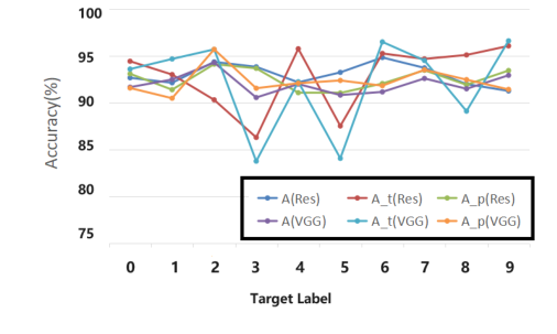Figure 3. Performance of different target label lp. We show the poison model accuracy (A), accuracy of target label (At), attack success rate (Ap) on CIFAR-10, using VGG16 and ResNet18