milliMamba: Specular-Aware Human Pose Estimation via Dual mmWave Radar with Multi-Frame Mamba Fusion

Background & Academic Lineage

The Origin & Academic Lineage

The problem of Human Pose Estimation (HPE) using millimeter-wave (mmWave) radar signals emerged primarily as a response to the limitations of traditional camera-based (RGB) systems. While RGB cameras provide rich visual information, they inherently raise privacy concerns, especially in sensitive environments like homes or hospitals. Furthermore, camera-based systems are susceptible to varying lighting conditions and occlusions, which can severely degrade performance.

In this context, mmWave radar presented itself as a compelling alternative. It offers a privacy-preserving solution because it doesn't capture visual images of individuals. Additionally, it's robust to environmental factors like darkness or smoke, making it suitable for a wider range of deployment scenarios. The specific problem addressed in this paper, therefore, is to develop a robust and accurate 2D human pose estimation system that leverages the unique advantages of mmWave radar while overcoming its inherent challenges.

The fundamental limitation or "pain point" of previous mmWave radar-based HPE approaches, which compelled the authors to develop milliMamba, stems from several issues. Firstly, radar signals are often sparse due to a phenomenon called "specular reflection." This means that signals might bounce away from the sensor if they hit a body part at certain angles, leading to incomplete observations and making it difficult to reconstruct a full-body pose from a single frame. Weak reflections from extremities (like fingers or toes) and sensitivity to subject orientation further exacerbate this problem. Secondly, prior methods, especially those based on Transformers, struggled with the high dimensionality of radar inputs and the large "token volumes" required for processing longer sequences of frames. This led to quadratic computational complexity, making them memory-intensive and slow. Some attempts to mitigate this involved "early fusion" of temporal information, but this often compromised the model's ability to recover missing joints by losing valuable contextual cues from neighboring frames. The authors' goal was to create a system that could efficiently process long sequences of radar data to leverage spatio-temporal context, thereby inferring missing joints more accurately and maintaining temporal consistency, all while keeping computational costs manageable.

Intuitive Domain Terms

• Millimeter-wave (mmWave) radar: Imagine a bat using its sonar to "see" in the dark, but instead of sound waves, we're using very short radio waves. These waves bounce off objects, and by listening to the echoes, we can figure out where things are and how they're moving, all without needing a camera. It's like having X-ray vision for motion, but without actually seeing the person.
• Human Pose Estimation (HPE): Think of it like drawing a stick figure over a person's body. The goal is to pinpoint the exact locations of key joints (like elbows, knees, and shoulders) to understand their posture and movement.
• Specular Reflection: This is like looking into a perfectly smooth mirror. If a radar signal hits a body surface that's very smooth and angled just right, the signal bounces off completely, like light off a mirror, and doesn't return to the radar sensor. This makes that part of the body "invisible" to the radar, leading to gaps in the data.
• Spatio-temporal Dependencies: This refers to how things are related both in space (where they are relative to each other at one moment) and time (how they move and change over a sequence of moments). For HPE, it means understanding that a person's arm movement in one frame is connected to its position in the previous and next frames, and also to the position of their shoulder.
• Mamba: This is a new type of artificial intelligence architecture, similar to a Transformer but much more efficient at handling long sequences of information. Imagine an incredibly smart note-taker who can quickly summarize and remember key points from a very long lecture without having to re-read the entire transcript every time. This allows the AI to understand context over much longer periods without getting overwhelmed.

Notation Table

Notation	Description

Problem Definition & Constraints

Core Problem Formulation & The Dilemma

The core problem addressed by this paper is 2D Human Pose Estimation (HPE) using millimeter-wave (mmWave) radar signals.

The Input/Current State for the proposed system consists of raw, complex-valued mmWave radar signals captured by dual radar sensors over a sequence of $T$ frames. Specifically, an FMCW radar produces complex-valued cubes $X \in C^{12 \times 128 \times 256}$ for each frame, corresponding to virtual-antenna pairs, chirps, and ADC samples. These raw signals are then preprocessed into 3D angle-doppler-range heatmaps, which are stacked across $T$ frames and split into real and imaginary components, forming a two-channel tensor of shape $C \times T \times H \times D \times W$ (where $C=2$). This input is inherently challenging due to its high dimensionality and the sparse nature of radar reflections.

The Output/Goal State is a sequence of temporally coherent 2D human poses, represented by the 2D keypoint coordinates for each joint across multiple frames within the sliding window. The objective is to accurately predict these joint coordinates, even for joints that are weakly reflected or entirely missing due to specular reflection, while maintaining temporal consistency and achieving state-of-the-art performance with reasonable computational complexity.

The exact missing link or mathematical gap that this paper attempts to bridge lies in the robust and efficient modeling of spatio-temporal dependencies from sparse, high-dimensional mmWave radar data. Previous methods struggle with:
1. Incomplete Observations: Specular reflections mean only body surfaces directly facing the receiver are captured, leading to missing or weakly reflected joints (especially extremities) and making full-body pose reconstruction from single-frame inputs diffcult.
2. Temporal Inconsistency: Fluctuations in radar signals disrupt temporal consistency across frames, hindering accurate pose estimation over time.
3. Computational Scalability: While Transformer-based models can capture global dependencies, their quadratic complexity with respect to sequence length makes them computationally expensive and memory-intensive for processing the large token volumes from longer radar sequences.
4. Partial Spatio-Temporal Modeling: Prior approaches often model spatio-temporal dependencies only partially or resort to early temporal fusion, which can compromise the model's ability to recover missing joints by discarding valuable contextual information.

The painful trade-off or dilemma that has trapped previous researchers is primarily between accuracy (especially for missing joints and temporal consistency) and computational efficiency/memory footprint. To achieve higher accuracy, especially in inferring missing joints and ensuring temporal smoothness, models need to process longer sequences and capture richer spatio-temporal context. However, traditional architectures like Transformers incur quadratic computational complexity and high memory demands for such long sequences, making them impractical. Conversely, methods that reduce complexity by early temporal fusion or single-frame prediction often sacrifice the contextual information necessary for robustly handling sparse, specular radar data and maintaining temporal consistency. This dilemma forces researchers to choose between a computationally expensive but potentially more accurate model, or a faster but less robust one.

Constraints & Failure Modes

The problem of mmWave radar-based human pose estimation is insanely diffcult due to several harsh, realistic walls the authors hit:

• Physical Constraints:

  • Specular Reflection: This is a primary challenge. Radar signals reflect off surfaces in a mirror-like fashion, meaning only body parts oriented directly towards the sensor are detected. This leads to extreme sparsity of data and incomplete observations, where small or obliquely oriented joints are often entirely missing from the radar data.
  • Weak Reflections from Extremities: Joints like wrists and ankles often produce very weak radar reflections, making them particularly hard to detect and track reliably.
  • Sensitivity to Subject Orientation and Sensor Placement: The quality and completeness of radar data are highly dependent on the subject's orientation relative to the sensors and the precise placement of the radar units, further complicating robust feature extraction.
  • Limited Elevation Resolution: mmWave radar sensors inherently have limited resolution in the elevation dimension, which can lead to ambiguities in 3D pose reconstruction. Dual-radar setups are used to mitigate this.

• Computational Constraints:

  • High Dimensionality of Radar Inputs: Raw radar signals are high-dimensional, and even after preprocessing into 3D heatmaps, the data volume for sequences of frames remains substantial.
  • Quadratic Complexity of Transformers: Prior Transformer-based models, while powerful for global dependency modeling, suffer from $O(N^2)$ complexity with respect to the input sequence length $N$. This makes them inefficient for processing the "large token volumes inherent in longer radar sequences," leading to prohibitive computational costs and training times.
  • Hardware Memory Limits: The quadratic complexity of Transformers directly translates to high memory consumption. As noted in the paper, Transformers "run out-of-memory on our hardware when trained with longer sequences" (e.g., beyond $T=3$ frames), severely limiting the amount of temporal context that can be processed.
  • Preprocessing Overhead: Traditional 4D heatmap generation from raw radar signals is computationally expensive and memory-intensive (e.g., 11x more memory and 8.6x more latency than 3D FFT-based heatmaps), which can be a bottleneck for real-time applications.

• Data-Driven Constraints:

  • Temporal Inconsistency: The inherent noise and fluctuations in radar signals can disrupt the temporal continuity of joint positions across frames, making it challenging to maintain smooth and consistent pose estimations over time.
  • Lack of Robust Features: Extracting robust and discriminative features from sparse and noisy radar signals is a significant hurdle, as the raw data does not directly provide visual cues like RGB images.
  • Difficulty in Inferring Missing Information: Due to specular reflections, the model must infer the positions of missing joints using contextual cues, which requires sophisticated spatio-temporal reasoning beyond simple per-frame analysis.

These constraints collectively make radar-based HPE a particularly challenging problem, demanding innovative architectural designs that can efficently handle high-dimensional, sparse, and temporally inconsistent data while maintaining computational tractability.

Why This Approach

The Inevitability of the Choice

When tackling the challenging problem of human pose estimation (HPE) using millimeter-wave (mmWave) radar, the authors faced a critical juncture where traditional state-of-the-art (SOTA) methods proved insufficient. The core issue stems from the inherent nature of radar signals: they are sparse due to specular reflections, leading to incomplete observations and missing joint data, especially from extremities. Furthermore, the raw radar inputs are high-dimensional, and the goal is to extract robust spatio-temporal features from longer sequences to infer these missing joints and ensure motion smoothness.

The authors explicitly recognized that prior Transformer-based approaches, while powerful for modeling global dependencies, suffered from a fatal flaw for this specific application: their quadratic complexity ($O(N^2)$) with respect to the input sequence length. As the paper states, processing the "large token volumes inherent in longer radar sequences" became an insurmountable challenge for Transformers due to their high computational costs, memory usage, and training time. For instance, Table 8 clearly shows that a Transformer encoder could only handle $T=3$ frames before running out of memory on their hardware, whereas the proposed Mamba-based encoder could scale to $T=9$ or even $T=15$ frames. This practical limitation meant Transformers simply couldn't process the necessary temporal context for robust pose estimation from radar.

Similarly, traditional CNN-based methods, while effective for capturing multi-scale spatial and short-term temporal features, were "often limited in their ability to fuse information from multiple radar sensors." Given that milliMamba utilizes a dual-radar setup for horizontal and vertical views, this limitation made standard CNNs a suboptimal choice.

The realization was clear: a new architecture was needed that could efficiently model long-range spatio-temporal dependencies with linear complexity ($O(N)$) to handle the high-dimensional, multi-frame radar data without prohibitive computational costs. This made the Mamba architecture, with its selective state space model (SSM) design, the only viable path forward.

Comparative Superiority

The milliMamba framework achieves qualitative superiority over previous gold standards primarily through its structural advantages in handling long sequences and complex spatio-temporal dependencies efficiently.

1. Linear Complexity for Long Sequences: The most significant structural advantage is the adoption of the Mamba architecture for the encoder. Unlike Transformers, which suffer from quadratic complexity $O(N^2)$ with sequence length $N$, Mamba offers linear complexity $O(N)$. This is not just a marginal improvement; it's a fundamental shift that allows milliMamba to process significantly longer radar sequences (e.g., $T=9$ frames by default, up to $T=15$ in experiments) without running out of memory, a critical limitation for Transformers as shown in Table 8. This enables the model to leverage much richer temporal context, which is crucial for inferring missing joints due to specular reflections and ensuring motion smoothness.

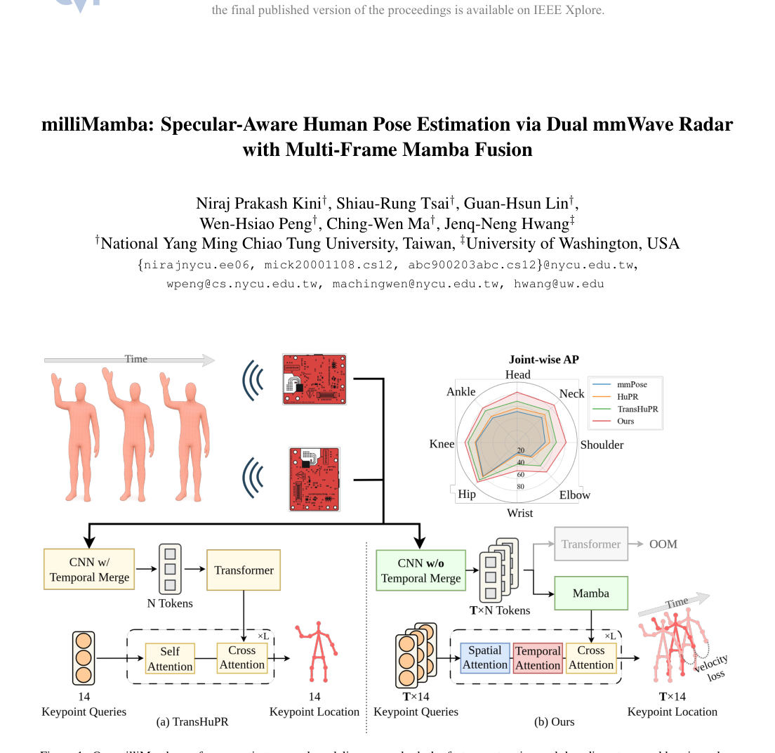Figure 1. Our milliMamba performs spatio-temporal modeling across both the feature extraction and decoding stages, addressing a key limitation of TransHuPR [12], which models these dependencies only partially. This is made possible by milliMamba’s ability to process a larger number of tokens with a comparable memory footprint, enabling richer temporal context and more accurate pose estimation

1. Enhanced Spatio-Temporal Context Modeling: The Cross-View Fusion Mamba (CV-Mamba) encoder is specifically designed to "capture dependencies over longer sequences efficiently" and "effectively fuses dual-radar inputs across frames." This allows for a more comprehensive understanding of the scene, which is vital for robust pose estimation from sparse radar data. Furthermore, the Spatio-Temporal-Cross Attention (STCA) decoder, with its multi-frame output strategy, integrates both spatial and temporal attention. This means it can model relationships within each frame (spatial) and across frames (temporal), leading to "richer supervision across time steps" and better inference of missing joints by leveraging contextual cues from neighboring frames and joints. This is a qualitative leap over methods that perform early temporal fusion or predict only a single frame.

2. Efficient Preprocesing: While not part of the core Mamba architecture, the choice of a 3D Fast Fourier Transform (FFT) for radar signal procesing significantly contributes to the overall superiority. As illustrated in Figure 4(c), this approach reduces memory usage by 11x and latency by 8.6x compared to the conventional 4D heatmap generation. This efficiency gain is crucial because it mitigates the "explosion of token counts," making the high-dimensional radar data tractable for downstream modeling by the Mamba encoder. This combined efficiency allows milliMamba to achieve higher accuracy with a more favorable balance between computational cost and performance, as highlighted in Tables 2 and 3.

In essence, milliMamba is overwelmingly superior because it provides a scalable, efficient, and context-rich framework that can process the extensive spatio-temporal information required for accurate radar-based HPE, a feat that prior methods struggled with due to architectural limitations.

Alignment with Constraints

The chosen milliMamba approach perfectly aligns with the harsh requirements of mmWave radar-based human pose estimation, forming a strong "marriage" between the problem's unique challenges and the solution's tailored properties.

1. Handling Sparse and Incomplete Data (Specular Reflection): The core problem is the sparsity of radar signals and missing joint information due to specular reflections. milliMamba addresses this head-on through its comprehensive spatio-temporal modeling. The CV-Mamba encoder extracts features from longer sequences, providing ample temporal context. The STCA decoder then leverages this context by predicting poses across multiple frames simultaneously and integrating both spatial and temporal attention. This enables the model to "leverage contextual cues from neighboring frames and joints to infer missing joints caused by specular reflections," directly mitigating the effects of incomplete observations. The velocity loss also reinforces motion smoothness, which helps in reconstructing plausible poses even when individual frames are sparse.

2. Managing High-Dimensional Inputs and Large Token Volumes: mmWave radar inputs are inherently high-dimensional. The milliMamba framework tackles this by first employing an efficient 3D FFT-based preprocessing step, which significantly reduces memory usage and latency compared to traditional 4D approaches (Figure 4(c)). This step "mitigates the explosion of token counts," making the data manageable. Subsequently, the CV-Mamba encoder, with its linear complexity, is specifically designed to "efficiently process the large token volumes inherent in longer radar sequences," a critical requirement that traditional Transformers failed to meet due to their quadratic scaling.

3. Fusing Multi-Radar Inputs: The problem often involves dual-radar setups to capture more comprehensive views. The CV-Mamba encoder is explicitly designed for "cross-view fusion of dual-radar inputs," effectively combining information from horizontal and vertical radar views. This directly addresses the need to integrate data from multiple sensors, a known limitation of some CNN-based methods.

4. Ensuring Temporal Consistency and Motion Smoothness: Weak reflections and fluctuations can disrupt temporal consistency. The multi-frame prediction strategy of the STCA decoder, combined with the explicit incorporation of a velocity loss ($L_{vel}$) during training, directly enforces motion consistency across frames. The velocity loss, defined as $L_{vel} = \frac{1}{T-1}\sum_{f=1}^{T-1}\sum_{j=1}^{J} ||\mathbf{v}_{f,j} - \hat{\mathbf{v}}_{f,j}||^2$, where $\mathbf{v}_{f,j}$ is the ground-truth velocity and $\hat{\mathbf{v}}_{f,j}$ is the predicted velocity, penalizes discrepancies in joint velocities, thereby promoting smooth and realistic pose sequences.

In summary, milliMamba's unique combination of efficient preprocessing, linear-complexity Mamba encoder for long-range spatio-temporal fusion, and a multi-frame attention decoder with velocity loss creates a robust and computationally feasible solution that directly addresses every major constraint of mmWave radar-based HPE.

Rejection of Alternatives

The paper provides clear reasoning for rejecting several popular alternative approaches, highlighting why milliMamba's design choices were necessary.

1. Transformers: The most prominent alternative, Transformers, were rejected primarily due to their quadratic computational complexity ($O(N^2)$) with respect to the input sequence length. The authors explicitly state that this makes them unsuitable for processing the "large token volumes inherent in longer radar sequences" required for robust radar-based HPE. Table 8 provides empirical evidence, showing that a Transformer encoder could not even process $T=9$ frames due to "out-of-memory issues" on their hardware, whereas Mamba handled it efficiently. This fundamental scalability issue made Transformers impractical for the problem's demands for extensive temporal context.

2. CNN-based Methods: While useful for some tasks, CNNs were deemed insufficient because they are "often limited in their ability to fuse information from multiple radar sensors." Given milliMamba's dual-radar input (horizontal and vertical views), a method with superior multi-sensor fusion capabilities was required, which Transformers (and subsequently Mamba) inherently offer through their attention/SSM mechanisms.

3. Early Temporal Fusion Approaches: Some prior methods [2, 12, 13] attempted to handle temporal information by "collapsing the temporal dimension early." The authors explicitly reject this strategy, arguing that "such early fusion can compromise the model's ability to recover missing joints caused by specular reflections." This is a critical qualitative rejection, as milliMamba's primary goal is to infer these missing joints by leveraging rich spatio-temporal context, which early fusion would diminish.

4. Many-to-one Prediction Strategy: Most prior radar-based HPE methods adopt a "multi-frame to single-frame decoding scheme," meaning they take multiple frames as input but predict only one pose (typically the central frame). milliMamba, in contrast, employs a "many-to-many" prediction strategy, outputting poses for multiple frames simultaneously. Table 5 quantitatively supports this rejection, showing that the "Many-to-one" strategy yields a significantly lower overall AP (70.4) compared to milliMamba's "Many-to-many" approach (74.5), a 4.1 AP improvement. This demonstrates the superior contextual inference capabilities of predicting multiple frames.

5. 4D Heatmap Preprocessing: The conventional approach of generating 4D heatmaps [25] from raw radar signals was rejected due to its computational inefficiency. The paper highlights that this method is "computationally expensive" and leads to an "explosion of token counts." Figure 4(c) provides a stark comparison, showing that 4D heatmap generation incurs 11x higher peak memory and 8.6x longer execution time compared to milliMamba's 3D FFT-based preprocessing. This clear inefficiency made the 4D approach unsuitable for a practical and scalable system.

These rejections underscore the authors' deep understanding of the problem's constraints and the limitations of existing techniques, leading them to develop milliMamba as a tailored and more effective solution. The choice of Mamba was not arbitrary but a necessity driven by the inherent incompatability of other SOTA models with the specific demands of mmWave radar data.

Mathematical & Logical Mechanism

The Master Equation

The mathematical core of milliMamba is driven by two principal sets of equations: the State Space Model (SSM) update equations, which form the backbone of the Cross-View Fusion Mamba (CVMamba) encoder, and the comprehensive training objective function that orchestrates the model's learning.

The SSM update for each Vision Mamba layer is defined as:
$$ h_{t+1} = A h_t + B u_t \\ y_t = C h_t + D u_t $$
where $t$ represents the time step.

The overall training objective, which the model strives to minimize during its learning phase, is:
$$ L = L_{oks} + \lambda_{vel} L_{vel} $$
The velocity loss, $L_{vel}$, is further specified as:
$$ L_{vel} = \frac{1}{(T-1)J} \sum_{f=1}^{T-1} \sum_{j=1}^{J} ||v_{f,j} - \hat{v}_{f,j}||^2_2 $$

Term-by-Term Autopsy

Let's meticulously break down each term within these equations to understand its mathematical definition, its physical or logical role, and the rationale behind its inclusion and form.

For the State Space Model (SSM) Update Equations:

• $h_t$:

  • Mathematical Definition: This is the hidden state vector of the SSM at time step $t$. It's a compact representation of the sequence's history up to the current point.
  • Physical/Logical Role: Conceptually, $h_t$ acts as the model's "memory" or "contextual summary." It accumulates and retains information from all preceding input tokens, enabling the model to understand and leverage long-range temporal dependencies within the radar data. Its evolution from $h_t$ to $h_{t+1}$ is central to sequential processing.
  • Why used: The authors employ this state-space formulation to achieve linear-time complexity for processing long sequences. This is a significant advantage over traditional Transformer architectures, which incur quadratic computational costs due to their global attention mechanisms, making them less suitable for the high-dimensional, multi-frame radar inputs.

• $u_t$:

  • Mathematical Definition: This is the input token vector at time step $t$. In milliMamba, these tokens are derived from the preprocessed radar heatmaps, representing spatio-temporal features from a specific moment in the sequence.
  • Physical/Logical Role: $u_t$ serves as the "current observation" or "new information" fed into the SSM at each step. It's the immediate piece of radar data that the model needs to integrate into its evolving understanding of the human pose.
  • Why used: It's the direct external stimulus that drives the SSM's state updates and contributes to the current output, providing the raw feature information from the radar.

• $y_t$:

  • Mathematical Definition: This is the output token vector generated by the SSM at time step $t$.
  • Physical/Logical Role: $y_t$ represents the transformed feature or immediate output at time $t$, which is a function of both the current input $u_t$ and the accumulated hidden state $h_t$. Within the Mamba layer, this output contributes to the overall encoded features that are subsequently passed to the decoder.
  • Why used: It provides a processed, context-aware representation of the input at time $t$, which can then be used by subsequent layers in the encoder or as the final output of the SSM block.

• $A, B, C, D$:

  • Mathematical Definition: These are layer-specific learnable parameter matrices (or sometimes vectors, depending on the specific SSM variant and dimensions). They are initialized and optimized during the training process.
  • Physical/Logical Role:
    • $A$: The state transition matrix. It governs how the previous hidden state $h_t$ propagates and transforms into the next hidden state $h_{t+1}$ intrinsically. It captures the inherent dynamics and persistence of information within the sequence, essentially defining how the "memory" evolves over time.
    • $B$: The input matrix. It determines how the current input $u_t$ is incorporated into the update of the hidden state $h_{t+1}$. It controls the influence of "new data" on the model's memory.
    • $C$: The output matrix. It transforms the hidden state $h_t$ into the output $y_t$. It's responsible for extracting relevant information from the model's memory to form the current output.
    • $D$: The direct feedthrough matrix. It allows the current input $u_t$ to directly contribute to the output $y_t$ without first being integrated into the hidden state. This can capture immediate, non-sequential relationships.
  • Why used: These matrices are the trainable components that allow the SSM to learn complex temporal dependencies and transformations from the radar data. Their values are optimized to best model the underlying dynamics of human motion. The use of addition and multiplication is fundamental to linear state-space systems, representing linear transformations and updates that are computationally efficient.

For the Overall Training Objective $L$:

• $L$:

  • Mathematical Definition: The scalar value representing the total loss that the model aims to minimize during training.
  • Physical/Logical Role: This is the primary feedback signal for the entire learning process. A lower value of $L$ signifies that the model's predictions are more accurate and temporally consistent according to the defined criteria. The model's parameters are iteratively adjusted to reduce this value.
  • Why used: It serves as the objective function that quantifies the "error" of the model's predictions, guiding the optimization process via gradient descent.

• $L_{oks}$:

  • Mathematical Definition: Object Keypoint Similarity (OKS) loss. While its exact formula isn't provided in the paper, it's a standard metric in human pose estimation, typically measuring the similarity between predicted and ground-truth keypoints, normalized by object scale and weighted by keypoint visibility.
  • Physical/Logical Role: This term directly assesses the spatial accuracy of the predicted 2D keypoint locations against the true positions. It ensures that the model learns to correctly identify and place human joints in each individual frame.
  • Why used: OKS is a widely adopted and robust loss function for pose estimation, directly reflecting the primary goal of the task. It's added to the velocity loss, indicating that both static pose accuracy and temporal smoothness are considered important and contribute independently to the overall error.

• $\lambda_{vel}$:

  • Mathematical Definition: A scalar weighting coefficient for the velocity loss term. The paper specifies $\lambda_{vel} = 0.05$.
  • Physical/Logical Role: This parameter acts as a dial to balance the importance of temporal smoothness (enforced by $L_{vel}$) against the raw keypoint accuracy (driven by $L_{oks}$). A small value like 0.05 suggests that while temporal consistency is valued, it should not overshadow the fundamental requirement of accurate keypoint prediction.
  • Why used: It provides a tunable hyperparameter, allowing the authors to fine-tune the model's behavior and achieve an optimal trade-off between different learning objectives.

• $L_{vel}$:

  • Mathematical Definition: The velocity loss, computed as the mean squared L2 norm of the difference between predicted and ground-truth joint velocities across all relevant frames and joints.
  • Physical/Logical Role: This term functions as a "temporal regularizer" or a "motion smoothness enforcer." It penalizes sudden, unrealistic changes in joint positions between consecutive frames, thereby promoting smooth and consistent motion in the predicted pose sequences. This is particularly beneficial for inferring missing joints caused by sparse radar signals or specular reflections, as the model is encouraged to predict plausible motion trajectories.
  • Why used: The authors introduced this loss to mitigate challenges posed by radar data, such as missing or noisy joint observations. By enforcing smoothness, the model can "fill in" gaps more realistically. The squared L2 norm ($||\cdot||^2_2$) is a standard choice for regression errors, penalizing larger deviations more significantly and providing a differentiable objective. The summation ($\sum$) aggregates errors across all consecutive frame pairs ($T-1$) and all joints ($J$), while the division by $(T-1)J$ normalizes the loss, making it independent of sequence length or number of joints.

• $T$:

  • Mathematical Definition: The total number of frames in the input sequence.
  • Physical/Logical Role: This dimension defines the temporal window over which the velocity loss is computed, establishing the extent of temporal context considered.
  • Why used: It's a fundamental parameter of the input data, dictating the length of the sequence being analyzed for motion.

• $J$:

  • Mathematical Definition: The total number of human body joints being estimated.
  • Physical/Logical Role: This dimension specifies the number of individual keypoints for which velocities are calculated and compared.
  • Why used: It's a fundamental parameter of the output data, representing the granularity of the human pose estimation.

• $f$:

  • Mathematical Definition: An index iterating over frames from $1$ to $T-1$.
  • Physical/Logical Role: This index pinpoints which specific pair of consecutive frames (frame $f$ and frame $f+1$) the velocity is being calculated for.
  • Why used: To systematically traverse and compute velocities across the temporal dimension of the sequence.

• $j$:

  • Mathematical Definition: An index iterating over joints from $1$ to $J$.
  • Physical/Logical Role: This index identifies which particular joint's velocity is currently under consideration.
  • Why used: To systematically traverse and compute velocities across the spatial dimension of the pose.

• $v_{f,j}$:

  • Mathematical Definition: The ground-truth velocity of joint $j$ at frame $f$. It's computed as the difference between its ground-truth positions at frame $f+1$ and frame $f$: $P_{f+1,j} - P_{f,j}$.
  • Physical/Logical Role: This represents the true, desired motion vector for a specific joint between two consecutive frames, serving as the ideal target for the model.
  • Why used: It provides the accurate reference against which the model's predicted motion is compared, guiding the learning process.

• $\hat{v}_{f,j}$:

  • Mathematical Definition: The predicted velocity of joint $j$ at frame $f$. It's calculated as the difference between its predicted positions at frame $f+1$ and frame $f$: $\hat{P}_{f+1,j} - \hat{P}_{f,j}$.
  • Physical/Logical Role: This is the model's estimated motion vector for a specific joint. Its deviation from the ground-truth velocity $v_{f,j}$ is what the velocity loss penalizes.
  • Why used: This is the output of the model's pose prediction for consecutive frames, which is then used to compute the velocity loss.

• $||\cdot||^2_2$:

  • Mathematical Definition: The squared Euclidean (L2) norm of a vector. For a vector $x = [x_1, x_2, \dots, x_k]$, its squared L2 norm is $||x||^2_2 = \sum_{i=1}^k x_i^2$.
  • Physical/Logical Role: This quantifies the squared magnitude of the difference vector between predicted and ground-truth velocities. Squaring ensures that both positive and negative differences contribute to the loss and that larger errors are penalized more significantly than smaller ones.
  • Why used: It's a standard, differentiable, and computationally efficient way to measure the "distance" or "error" between two vectors, making it well-suited for gradient-based optimization.

Step-by-Step Flow

Let's trace the journey of an abstract data point, from raw radar signals to a refined pose prediction, as it moves through the milliMamba's mechanical assembly line.

1. Raw Radar Signal Ingestion: The process begins with raw millimeter-wave (mmWave) radar signals. These arrive as complex-valued cubes $X \in \mathbb{C}^{12 \times 128 \times 256}$ for each frame, representing data across virtual-antenna pairs, chirps, and ADC samples. Since milliMamba uses a dual-radar setup, two such cubes (one for horizontal, one for vertical view) are acquired for a sequence of $T$ consecutive frames, forming a sliding window of temporal context.

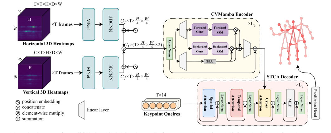Figure 2. Overview of our milliMamba. The CVMamba encoder first extracts features from dual-view radar inputs. These features are then passed to the Multi-Pose STCA decoder, which progressively refines a set of keypoint queries to produce pose predictions

1. Pre-processing Assembly Line (3D Fast Fourier Transform):
   • Clutter Removal: First, static reflections from the environment are filtered out by subtracting the mean across chirps. This is like cleaning the raw material, ensuring only relevant moving targets are processed.
   • Chirp Sub-sampling: The chirp dimension is then uniformly reduced to 8 chirps per frame. This step is akin to compressing the data, reducing computational load while preserving essential Doppler resolution.
   • 1D FFT (Range): A 1D Fast Fourier Transform (FFT) is applied along the ADC-sample dimension (as per $Y(m) = \sum_{n=0}^{N-1} X(n) \exp(-j \frac{2\pi nm}{N})$). This transforms the raw time-domain samples into range information, indicating the distance of objects.
   • 1D FFT (Doppler): Next, another 1D FFT is applied along the chirp dimension. This extracts Doppler information, which reveals the velocity of objects relative to the radar.
   • Zero-Padding & 1D FFT (Angle): To enhance angular resolution, the virtual-antenna dimension is zero-padded from 12 to 64. A final 1D FFT along this dimension converts the data into angle information (azimuth and elevation).
   • Output: The radar data for each view and frame is now a 3D angle-doppler-range heatmap $Y \in \mathbb{C}^{H \times D \times W}$ (e.g., $64 \times 8 \times 256$). The real and imaginary components of these complex-valued heatmaps are treated as separate channels, resulting in a two-channel tensor of shape $C \times T \times H \times D \times W$ where $C=2$.

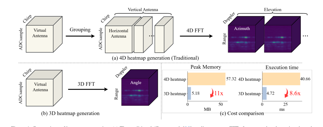Figure 4. Comparison of heatmap generation. (a) The traditional 4D approach [25] applies separate FFTs for range, doppler, azimuth, and elevation after antenna grouping. (b) Our 3D pipeline performs a unified spatial FFT without grouping, yielding a compact representation. (c) Cost comparison between 4D and 3D heatmaps, showing 11× reduction in memory and 8.6× reduction in latency

1. CVMamba Encoder - Feature Extraction & Temporal Modeling:

   • Parallel MNet Branches: The horizontal and vertical view heatmaps are fed into two distinct, parallel MNet blocks. Each MNet block first merges the Doppler dimension, then processes the data through a series of residual 3D convolutions and down-sampling layers. This reduces the spatial resolution (H and W) by a factor of $4 \times$, yielding feature maps $F_h, F_v \in \mathbb{R}^{C_f \times T \times \frac{H}{4} \times \frac{W}{4}}$. This is like two specialized parallel processing lines handling different perspectives.
   • Positional Embeddings: Separate learnable positional embeddings $P_h$ and $P_v$ are added to $F_h$ and $F_v$, respectively. These embeddings inject information about the absolute spatial location (angle and range) of the features into the data.
   • Cross-View Fusion: The two view features are then concatenated along a channel dimension to form the unified encoder input $F = [F_h; F_v] \in \mathbb{R}^{C_s \times T \times \frac{H}{4} \times \frac{W}{4} \times 2}$. This step effectively merges the information from both radar views.
   • Sequence Linearization: The multi-dimensional feature tensor $F$ is then converted into a 1D sequence of tokens $u_t$ using a specific zigzag scan pattern (range $\rightarrow$ angle $\rightarrow$ view $\rightarrow$ frame). This transformation prepares the data for the sequential processing of the Mamba architecture.
   • Mamba Layer Processing: This 1D sequence $u_t$ enters a stack of Vision Mamba layers. Each layer iteratively updates its hidden state $h_t$ and produces an output $y_t$ using the SSM equations ($h_{t+1} = A h_t + B u_t$, $y_t = C h_t + D u_t$). This process is executed in both forward and backward directions, allowing the model to efficiently capture bidirectional context over the entire long sequence with linear complexity. Gating mechanisms and residual connections within the Mamba layers further refine this sequential processing.
   • Output: The CVMamba encoder outputs a rich, context-aware feature representation, denoted as $x_{Le}$, which has effectively captured complex spatio-temporal dependencies across multiple frames and dual radar views.

2. STCA Decoder - Pose Prediction & Refinement:

   • Keypoint Query Initialization: The decoder begins with a fixed set of $J \times T$ learnable keypoint queries $\{q_{f,j}\}$. Each query is an embedding designed to represent a specific joint in a specific frame. These queries act like "intelligent probes" searching for pose information.
   • Spatio-Temporal Attention Module:
     • Spatial Attention (SA): First, spatial self-attention is applied within each frame ($q'_{f,.} = \text{softmax}(Q_f K_f^T / \sqrt{d}) V_f$). This allows queries for different joints within the same frame to interact, capturing inter-joint relationships (e.g., how the elbow relates to the wrist in a single snapshot).
     • Temporal Attention (TA): Next, temporal self-attention is applied across frames for the same joint ($q''_{.,j} = \text{softmax}(Q_j K_j^T / \sqrt{d}) V_j$). This enables queries for a specific joint to attend to its own representation in neighboring frames, enforcing motion consistency and leveraging temporal context to understand movement.
   • Cross-Attention to Encoder Features: The refined keypoint queries $q''_{f,j}$ then perform cross-attention with the encoder's output features $F'$ (which is $x_{Le}$) ($\hat{q}_{f,j} = \text{CrossAttn}(q''_{f,j}, F')$). This crucial step allows the keypoint queries to extract relevant pose information from the rich spatio-temporal features generated by the CVMamba encoder, effectively "grounding" the queries in the radar data.
   • Iterative Refinement: This entire decoder layer (comprising Spatio-Temporal Attention, Cross-Attention, and a position-wise MLP) is stacked multiple times. The keypoint queries are iteratively refined through these layers, progressively improving their representation and accuracy.
   • Prediction Head: Finally, each refined query $\hat{q}_{f,j}$ is passed through a simple prediction head (e.g., a multi-layer perceptron) to output the 2D coordinates for joint $j$ in frame $f$.
   • Output: The decoder produces a sequence of $T$ pose estimates, where each estimate consists of $J$ 2D keypoint coordinates. During inference, typically only the prediction for the central frame within the sliding window is retained.

Optimization Dynamics

The milliMamba model learns and refines its human pose estimation capabilities through a rigorous process of iterative optimization, primarily guided by the overall training objective $L = L_{oks} + \lambda_{vel} L_{vel}$. This mechanism systematically adjusts the model's internal parameters to minimize the disparity between its predictions and the ground truth.

1. Loss Landscape and Gradient Behavior:

   • The total loss $L$ defines a complex, high-dimensional "loss landscape" over the vast space of all learnable model parameters. The fundamental goal of the optimization process is to navigate this landscape to locate its lowest point (global minimum) or a sufficiently low point (local minimum).
   • $L_{oks}$ (Object Keypoint Similarity Loss): This component of the loss function primarily shapes the landscape to reward accurate spatial placement of individual keypoints. It generates gradients that effectively "pull" predicted keypoints closer to their corresponding ground-truth locations. If a predicted keypoint is significantly displaced from its true position, $L_{oks}$ will produce a strong gradient, compelling the model to adjust its parameters to reduce this spatial error.
   • $L_{vel}$ (Velocity Loss): This component introduces a vital regularization effect, sculpting the loss landscape to favor temporally smooth and consistent pose sequences. It generates gradients that actively penalize abrupt or unrealistic changes in joint positions between consecutive frames. If a joint's predicted velocity deviates substantially from the ground-truth velocity, $L_{vel}$ will produce gradients that encourage the model to predict smoother, more physically plausible motion. This is particularly beneficial for inferring missing joints caused by sparse radar signals or specular reflections, as the model learns to "interpolate" plausible motion based on contextual cues from neighboring frames.
   • Balancing Act ($\lambda_{vel}$): The weighting factor $\lambda_{vel}$, set to a value of 0.05, plays a critical role in balancing the importance of temporal smoothness (enforced by $L_{vel}$) against the primary objective of raw keypoint accuracy (driven by $L_{oks}$). This relatively small value ensures that while temporal consistency is an important consideration, it does not overpower the fundamental requirement of accurate keypoint prediction. Consequently, the gradients originating from $L_{oks}$ will generally exert a stronger influence, guiding the model towards precise pose estimations, while $L_{vel}$ provides a gentle, yet persistent, pull towards temporal coherence. Without $L_{vel}$, the model might produce accurate but jerky poses; with an excessively high $\lambda_{vel}$, it might prioritize smoothness at the expense of accuracy.

2. Iterative State Updates:

   • Forward Pass: During each training iteration, a batch of multi-frame radar sequences is fed through the entire milliMamba network—encompassing the pre-processing, CVMamba encoder, and STCA decoder. This forward propagation culminates in the generation of a sequence of predicted 2D keypoint coordinates $\hat{P}_{f,j}$ for each frame $f$ and joint $j$.
   • Loss Calculation: These predicted keypoint coordinates are then rigorously compared against the ground-truth keypoint coordinates $P_{f,j}$ to compute $L_{oks}$. Concurrently, predicted velocities $\hat{v}_{f,j}$ (derived from $\hat{P}_{f,j}$) are compared with ground-truth velocities $v_{f,j}$ (derived from $P_{f,j}$) to calculate $L_{vel}$. These two distinct loss components are then combined according to the master equation: $L = L_{oks} + \lambda_{vel} L_{vel}$.
   • Backward Pass (Backpropagation): The calculated total loss $L$ is subsequently backpropagated through the entire network. This intricate process computes the gradients of $L$ with respect to every single learnable parameter within the model. This includes, for instance, the matrices $A, B, C, D$ in the Mamba layers, the weights of the convolutional neural networks (CNNs) in the MNet blocks, the attention matrices in the STCA decoder, and the initial learnable keypoint queries.
   • Parameter Update (Adam Optimizer): An Adam optimizer is employed to update the model's parameters. Adam is an advanced adaptive learning rate optimization algorithm that computes individual adaptive learning rates for different parameters based on estimates of the first and second moments of the gradients. With a specified learning rate of 0.00005 and a weight decay of 0.0001, the optimizer intelligently adjusts the parameters in the direction that most effectively reduces the loss. The weight decay term acts as a regularization mechanism, helping to prevent the model from becoming overly complex and overfitting the training data.
   • Convergence: This cyclical process of forward pass, loss calculation, backward pass, and parameter update is repeated for numerous epochs (iterations over the entire training dataset). Over time, the model's parameters gradually converge to values that minimize the loss function, leading to progressively improved pose estimation accuracy and enhanced temporal consistency on both the training data and previously unseen data. The iterative refinement steps embedded within the STCA decoder itself also contribute significantly to this convergence, as the keypoint queries are progressively updated to better represent the underlying pose. The model's performance on a separate validation set is continuously monitored to detect signs of overfitting and to determine the optimal point at which to halt training.

Results, Limitations & Conclusion

Experimental Design & Baselines

To rigorously validate milliMamba's capabilities, the authors architected a series of experiements designed to isolate and quantify the contributions of their proposed mechanisms. The core setup involved feeding dual millimeter-wave (mmWave) radar inputs, each capturing a sequence of $T=9$ frames, into the model. While the model produced 9 consecutive pose predictions, only the central frame's prediction was ultimately used for inference, ensuring a fair comparison with methods that predict a single pose per input.

The training regimen utilized the Adam optimizer with a learning rate of 0.00005, a batch size of 8, and a weight decay of 0.0001. The overall training objective was a composite loss function: $L = L_{oks} + \lambda_{vel} L_{vel}$. Here, $L_{oks}$ (Object Keypoint Similarity) penalized discrepancies between predicted and ground-truth joint locations, a standard metric in pose estimation. Crucially, $L_{vel}$ (velocity loss) was introduced to enforce temporal smoothness by minimizing the error between predicted and ground-truth joint velocities, with a weighting factor $\lambda_{vel} = 0.05$. This velocity loss was a key architectural choice to address the temporal inconsistency often seen in radar-based pose estimation. All computational heavy lifting was performed on a single NVIDIA Tesla V100 GPU.

The "victims" (baseline models) against which milliMamba was pitted included established radar-based 2D Human Pose Estimation (HPE) methods:
- TransHuPR [12]: A Transformer-based approach that partially models spatio-temporal dependencies.
- HuPR [13]: Another prominent radar-based HPE framework.
- mmPose [23]: A CNN-based method.
The authors also acknowledged RFMamba [35], another Mamba-based approach, but noted its source code was not publicly available, precluding direct comparison.

Evaluation was conducted on two benchmark mmWave radar-based 2D HPE datasets:
- TransHuPR [12]: Comprising 440 sequences (over 7 hours) from 22 subjects, this dataset is characterized by fast and dynamic actions, posing a significant challenge.
- HuPR Dataset [13]: Containing 235 sequences (approximately 4 hours) from 6 subjects, this dataset primarily features relatively static actions.
For both datasets, standard data split protocols were followed. The definitive metric for evaluation was Average Precision (AP), calculated based on Object Keypoint Similarity (OKS). This included overall AP (averaged over OKS thresholds from 0.50 to 0.95), as well as AP50 (OKS 0.50) and AP75 (OKS 0.75) for loose and strict matching criteria, respectively.

What the Evidence Proves

The evidence presented in the paper provides undeniable proof that milliMamba's core mechanisms work in reality, leading to significant performance gains over existing baselines.

First, in terms of overall performance, milliMamba consistently and substantially outperformed all baselines across both the TransHuPR and HuPR datasets. On the challenging TransHuPR dataset, milliMamba achieved a remarkable 11.0 AP improvement over the TransHuPR [12] baseline. This was particularly evident for difficult-to-estimate joints like the wrist, which is prone to fast movement and specular reflections, where milliMamba achieved an AP of 46.9. Similarly, on the HuPR dataset, milliMamba delivered an even more impressive 14.6 AP improvement over HuPR [13], reaching up to 84.0 AP for relatively static actions. These numbers are not just incremental; they represent a significant leap in the state-of-the-art for radar-based HPE.

The paper also provides hard evidence for the efficiency and effectiveness of its architectural choices:
- Efficient 3D FFT Preprocessing: Figure 4(c) definitively shows that the proposed 3D Fast Fourier Transform (FFT) preprocessing pipeline reduces memory usage by 11x and latency by 8.6x compared to the conventional 4D FFT approach. Table 4 further validates this by demonstrating that 3D FFT-based heatmaps achieve comparable, if not superior, accuracy (74.5 AP) to 4D FFT (72.0 AP), proving that efficiency gains did not come at the cost of performance.
- Multi-Pose Output Mechanism (Many-to-many): Table 5 clearly illustrates the benifit of milliMamba's Spatio-Temporal-Cross Attention (STCA) decoder. The "Many-to-many" prediction strategy, which leverages contextual cues from neighboring frames, yielded a 4.1 AP improvement in overall accuracy compared to a "Many-to-one" approach (a vanilla Transformer decoder predicting a single pose). This is definitive proof that modeling spatio-temporal dependencies in the decoding stage is crucial for inferring missing joints due to specular reflections.
- Mamba Encoder's Scalability: The comparison between Mamba and Transformer encoders in Table 8 is particularly compelling. While Mamba achieved a 1.5 AP higher score than Transformer for short sequences ($T=3$ frames), the critical evidence lies in the Transformer's inability to handle longer sequences due to out-of-memory issues. Mamba, with its linear complexity, scales succesfully to longer input sequences (up to $T=15$ frames, as shown in Table 6), where performance consistently improves. This demonstrates Mamba's superior scalability and its ability to effectively leverage richer temporal context, a key claim of the paper.
- Dual-Radar Configuration: Table 7 provides clear evidence that the dual-radar (Horizontal+Vertical) configuration significantly boosts performance (78.5 AP) compared to using a single horizontal (67.3 AP) or vertical (74.5 AP) radar alone. This confirms the effectiveness of cross-view fusion in compensating for the inherent limited elevation resolution of mmWave radar sensors.

Qualitative results in Figure 5 further reinforce these findings, visually showcasing milliMamba's ability to produce more accurate and temporally consistent pose estimations across various actions on the TransHuPR dataset, outperforming mmPose, HuPR, and TransHuPR baselines.

Limitations & Future Directions

While milliMamba presents a significant advancement in radar-based human pose estimation, it's important to acknowledge its current limitations and consider avenues for future development.

One inherent limitation, despite milliMamba's efficiency improvements over traditional Transformers for long sequences, is the computational cost. While it offers a favorable trade-off between accuracy and complexity, its MACs count (34.4 G) is still higher than some baselines like TransHuPR [12] (5.8 G). This suggests that for deployment on highly resource-constrained edge devices, further optimization in terms of computational footprint might be necessary.

Another clear limitation is the current focus on single-person pose estimation. The paper explicitly states that future work will explore "multi-person" scenarios. Radar signals become significantly more complex with multiple subjects due to occlusions, interference, and the challenge of associating radar points with specific individuals. The current architecture, while robust for single persons, would likely require substantial modifications to handle the complexities of multi-person interactions.

Furthermore, the evaluation was conducted on two specific datasets, TransHuPR and HuPR, which represent certain types of actions and environments (implied to be indoor). While radar is robust to lighting conditions, the generalizability of milliMamba to diverse, unconstrained cross-environment scenarios (e.g., outdoor settings with varying clutter, different building materials, or more complex human-object interactions) remains an open question. The paper's mention of "cross-environment scenarios" in future work highlights this as an area needing further investigation.

Looking ahead, several exciting discussion topics emerge for further developing and evolving these findings:

1. Robust Multi-Person Pose Estimation: How can milliMamba's spatio-temporal modeling be extended to robustly handle multiple individuals? This could involve novel instance segmentation techniques for radar data, graph-based approaches to model inter-person relationships, or even incorporating prior knowledge about human group dynamics. What architectural changes would be needed to maintain linear complexity while scaling to many people?
2. Real-time Edge Deployment & Efficiency: Given the computational cost, what further architectural optimizations (e.g., quantization, pruning, knowledge distillation) could make milliMamba suitable for real-time inference on low-power edge devices? Could a more lightweight Mamba variant or a hybrid architecture offer a better balance for practical applications?
3. 3D Pose Estimation from 2D Heatmaps: The current work focuses on 2D HPE. How can the rich spatio-temporal features extracted by milliMamba be leveraged or extended to infer full 3D human poses? This would likely involve adapting the output head and potentially incorporating additional geometric constraints or multi-view fusion strategies to resolve depth ambiguities inherent in 2D projections.
4. Enhanced Specular Reflection Handling: While milliMamba addresses specular reflections, could more explicit physics-informed neural networks or advanced signal processing techniques be integrated into the Mamba encoder to directly model and compensate for these challenging radar phenomena? This might involve learning to distinguish direct reflections from specular ones or using generative models to "fill in" missing data caused by signal sparsity.
5. Longer-Term Temporal Context & Action Recognition: The Mamba encoder's ability to handle longer sequences is a key advantage. How can this be further exploited to not only improve pose estimation but also enable more sophisticated action recognition or activity understanding over extended periods? This could involve integrating recurrent mechanisms or hierarchical temporal modeling within the Mamba framework.
6. Fusion with Other Privacy-Preserving Modalities: While radar is privacy-preserving, could fusing milliMamba with other non-RGB sensors (e.g., thermal cameras, depth sensors, or even acoustic sensors) provide complementary information to further enhance robustness in extremely challenging scenarios or for specific applications like medical monitoring or fall detection? What are the optimal fusion strategies for such diverse data types?

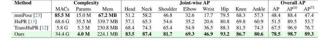Table 2. Comparison of model performance and complexity across methods on the TransHuPR dataset [12]. The complexity excludes radar signal preprocessing 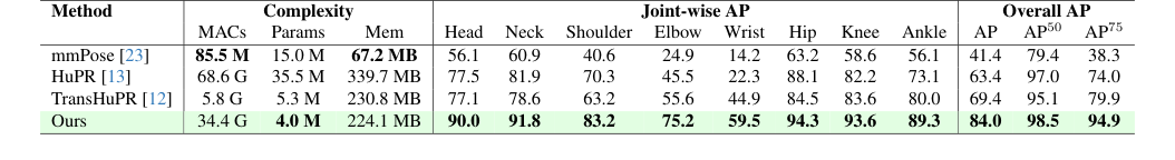Table 3. Comparison of model performance and complexity across methods on the HuPR dataset [13]. The complexity excludes radar signal preprocessing 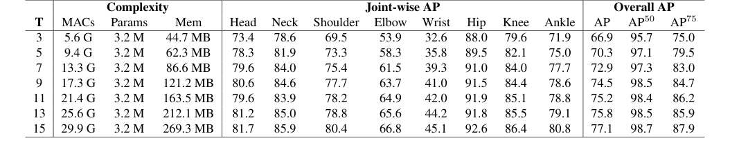Table 6. Impact of input sequence length (T) on pose estimation performance. We investigate the effect of varying T to understand how temporal context contributes to accuracy 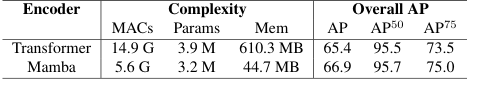Table 8. Comparison of Transformer and Mamba encoders with 3- frame radar inputs. Transformer runs out-of-memory on our hard- ware when trained with longer sequences