Learning to increase matching efficiency in identifying additional b-jets in the process
To truly understand the significance of this paper, we have to travel back to the monumental discovery of the Higgs boson at the Large Hadron Collider (LHC) in 2012.
Background & Academic Lineage
To truly understand the significance of this paper, we have to travel back to the monumental discovery of the Higgs boson at the Large Hadron Collider (LHC) in 2012. Once physicists found the Higgs, the next immediate question was: Does it behave exactly the way our standard models predict?
To answer this, scientists look at how the Higgs boson interacts with the heaviest known particle, the top quark. They specifically study a collision event called the $t\bar{t}H$ process, where a top quark pair ($t\bar{t}$) is produced alongside a Higgs boson ($H$). Because the Higgs boson most frequently decays into a pair of bottom quarks ($b\bar{b}$), the final debris we actually detect in the collider is a $t\bar{t}b\bar{b}$ signature.
Here is where the massive headache begins. The universe naturally produces $t\bar{t}b\bar{b}$ events through standard, non-Higgs physics processes. This non-Higgs $t\bar{t}b\bar{b}$ production acts as massive background noise. To find the rare Higgs "signal," physicists must perfectly understand this background. To do that, they need to look at the final debris and distingush which bottom quarks came from the top quarks, and which ones were "additional" bottom quarks generated by a random quantum event called gluon splitting.
The Fundamental Limitation of Previous Approaches
Prior to this paper, researchers tried to solve this identification problem using standard machine learning, specifically binary classification. They would take every single pair of $b$-jets in an event and ask the neural network: "Is this pair the additional one? Yes or No?"
The fundamental pain point here is that this approach completely ignores the physical stucture of the data. In almost every collision event, there is exactly one pair of additional $b$-jets. By evaluating each pair in total isolation, previous models were optimizing for overall "pair accuracy" rather than "event accuracy." Imagine grading a multiple-choice test by asking a computer to independently guess if A is right, if B is right, and if C is right, rather than forcing it to pick the single best answer out of the options. Because the old models didn't look at the whole event context simultaneously, their ability to correctly identify the one true pair per event (a metric called "matching efficiency") hit a hard ceiling.
Translating the Jargon
To make this intuitive, let's break down some highly specialized terms used in the paper:
- $b$-jet: When a bottom ($b$) quark is created in a particle collision, it decays almost instantly into a cone-shaped spray of other particles.
- Analogy: Think of a $b$-jet as a unique set of muddy footprints left behind by an invisible animal. We can't see the animal (the quark), but we can measure the footprints (the jet) to figure out where it came from.
- Gluon splitting: A quantum process where a gluon (a particle that carries the strong nuclear force) spontaneously transforms into a quark and an antiquark pair.
- Analogy: Imagine a single firework shell shooting into the sky and suddenly bursting into exactly two distinct, brightly colored sparks.
- Irreducible background: A background noise process that results in the exact same final detectable particles as the rare signal you are actually looking for.
- Analogy: Trying to tell if a cake was sweetened with white sugar or brown sugar just by looking at the final baked cake. The end result looks identical, so you have to look for incredibly subtle clues in the texture to tell them apart.
- Matching efficiency: The percentage of total collision events where the algorithm successfully identifies the exact correct pair of additional $b$-jets, rather than just getting a high average score on individual guesses.
- Analogy: A sniper's "one shot, one kill" metric. It doesn't matter if you correctly identify 99 innocent bystanders as "not the target"; what matters is if you can pick out the one specific target hidden in the crowd perfectly.
The Mathematical Problem and Solution
The authors wanted to directly maximize the matching efficiency. Mathematically, this is represented by the Kronecker delta function:
$$ \text{Matching efficiency} = \frac{1}{N} \sum_{i=1}^{N} \delta(y_i, \hat{y}(M_i)) $$
Here, $\delta(y_i, \hat{y}(M_i))$ equals $1$ if the model's prediction $\hat{y}$ perfectly matches the true index $y_i$, and $0$ otherwise.
The mathematical problem is that this function is a "hard step" (it jumps instantly from 0 to 1). In a machine learning enviornment, you cannot train a neural network on a hard step because the gradient (the slope used to update the network's weights) is zero almost everywhere. You can't use calculus to optimize it.
To overcome this constraint, the authors abandoned the old binary cross-entropy loss ($L_{BCE}$) and designed surrogate loss functions ($L_1, L_2, L_3, L_4$). They transformed the neural network's output into a probability distribution over all pairs in a given event using a softmax function:
$$ f_j(M_i) = \frac{\exp(g_j(M_i))}{\sum_{k=1}^{c_i} \exp(g_k(M_i))} $$
This equation forces the model to look at all $c_i$ pairs in the event matrix $M_i$ and assign them probabilities that sum to 1. Then, they train the model to maximize the probability assigned to the correct pair using a categorical cross-entropy surrogate loss, such as $L_3$:
$$ L_3 = - \frac{1}{N} \sum_{i=1}^{N} \log f_{y_i}(M_i) $$
By doing this, the model learns to rank the pairs against each other within the context of the specific event, directly optimizing toward the matching efficiency without breaking the rules of gradient descent.
Key Mathematical Notations
| Notation | Type | Description |
|---|---|---|
| $N$ | Parameter | The total number of simulated $t\bar{t}b\bar{b}$ event data samples. |
| $c_i$ | Variable | The total number of $b$-jet pairs present in the $i$-th event. |
| $F$ | Parameter | The dimension of the feature vector representing a single $b$-jet pair. |
| $M_i$ | Variable | The event matrix for the $i$-th event, containing all $b$-jet pairs, with dimensions $\mathbb{R}^{c_i \times F}$. |
| $y_i$ | Variable | The true integer index (from $1$ to $c_i$) indicating the actual pair of additional $b$-jets in the $i$-th event. |
| $\hat{y}(M_i)$ | Variable | The predicted index of the additional $b$-jet pair outputted by the model. |
| $f_j(M_i)$ | Variable | The model's predicted probability that the $j$-th $b$-jet pair in event $M_i$ is the additional pair. |
| $g_j(M_i)$ | Variable | The raw activation value (score) computed by the neural network for the $j$-th $b$-jet pair before being converted to a probability. |
| $L_{BCE}$ | Function | The traditional Binary Cross-Entropy loss used by previous, limited models. |
| $L_1, L_2, L_3, L_4$ | Function | The proposed surrogate loss functions designed to smoothly approximate and maximize matching efficiency. |
Problem Definition & Constraints
To understand the magnitude of the problem this paper tackles, imagine you are trying to listen to a very faint, specific whisper in a crowded, noisy staduim. In the world of particle physics, that whisper is the Higgs boson, a fundamental particle that gives mass to everything in the universe. However, when physicists smash protons together at the Large Hadron Collider (LHC) to study the Higgs boson, they are deafened by a massive amount of background noise.
The loudest noise comes from a physical process called $t\bar{t}b\bar{b}$, which produces a top quark pair alongside a bottom quark ($b$) pair. The debris from this process looks almost exactly like the debris from the Higgs boson. To filter out this noise, physicists must look at the resulting "b-jets" (sprays of particles) and figure out their origin story: did these b-jets come from the heavy top quarks decaying, or did they just pop into existence from a secondary process called "gluon splitting"?
The Starting Point and The Goal State
The Input (Current State):
When a particle collision (an "event") occurs, detectors capture the kinematic properties of the debris. The authors represent this data mathematically as an event matrix $M_i \in \mathbb{R}^{c_i \times F}$. Here, $c_i$ represents the number of possible b-jet pairs in a single collision event, and $F$ represents the high-dimensional physical features (like momentum and energy) of each pair.
The Output (Goal State):
The desired endpoint is a neural network that can look at this matrix and point to exactly one specific row, confidently declaring: "This specific pair of b-jets is the additional pair created by gluon splitting."
The Mathematical Gap:
The missing link is a specialized mathematical bridge that evaluates the b-jet pairs relative to one another within the same event. We don't just want to know if a pair looks like an additional b-jet in isolation; we need the network to rank all pairs in the matrix $M_i$ and output a probability distribution $f(M_i) \in [0, 1]^{c_i}$ where the probabilities sum to 1. The highest probability indicates the correct pair.
The Painful Dilemma
Previous researchers fell into a classic machine learning trap: they treated this as a standard binary classification problem. They took every single b-jet pair from every event, mixed them all together, and asked a neural network to guess "Yes" or "No" using a standard Binary Cross-Entropy loss function ($L_{BCE}$).
This created a painful trade-off between computational convenience and physical reality. Binary classification is mathematically easy to optimize, but it completely ignores the structural reality of the physics: almost every $t\bar{t}b\bar{b}$ event contains exactly one true pair of additional b-jets. By evaluating each pair in a vacuum, previous models threw away vital contextual clues.
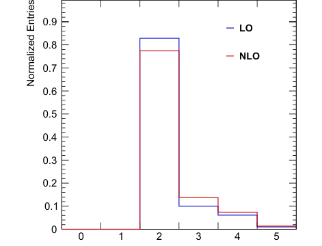 Figure 4. Histograms for the number of generator-level additional b-jets in simulated t¯tb¯b events at both the leading order (LO) and the next-to-leading order (NLO). Note that most events have two additional b-jets (82.8% for LO and 77.4% for NLO)
However, if you try to fix this by abandoning binary classification and directly optimizing for what you actually care about—the "matching efficency," which is the percentage of total events where the model picks the exact right pair—you immediately break the math. You are forced to choose between a model that is easy to train but structurally flawed, or a model that is structurally accurate but mathematically impossible to train.
The Harsh Walls and Constraints
What makes this problem insanely difficult to solve? The authors hit several massive walls:
1. The Non-Differentiable Wall (The Mathematical Constraint)
The ultimate goal is to maximize matching efficiency, which is mathematically defined as:
$$ \text{Matching efficiency} = \frac{1}{N} \sum_{i=1}^{N} \delta(y_i, \hat{y}(M_i)) $$
Here, $\delta$ is the Kronecker delta function. This function is a harsh, rigid staircase: it equals $1$ if the model's prediction $\hat{y}$ exactly matches the true label $y_i$, and $0$ otherwise. In calculus, the derivative (gradient) of a flat step is zero. Neural networks learn by following gradients (gradient descent). Because the Kronecker delta is highly non-differntiable and returns zero gradients almost everywhere, the neural network is left completely blind. It cannot learn because the math provides no directional feedback on how to improve.
2. Variable Data Structures (The Computational Constraint)
Every quantum collision is uniquely chaotic. One event might produce 3 pairs of b-jets, while the next produces 6. This means the input matrix $M_i$ has a constantly changing number of rows ($c_i$). The neural network architecture must be dynamically flexible enough to handle variable-sized inputs without crashing, while also being permutation-equivariant (meaning the order in which the b-jet pairs are fed into the model shouldn't change the model's underlying logic).
3. Extreme Quantum Complexity (The Physical Constraint)
There are no simple, hard-coded physics rules to separate these jets. The data is generated by highly complex, stochastic quantum processes. Hand-engineering features is practically impossible. The kinematic observables are deeply entangled, meaning the model must somehow learn to untangle high-dimensional relationships purely from simulated data, without any explicit human-made rules to guide it.
Why This Approach
To understand why the authors took this specific mathematical route, we have to pinpoint the exact moment they realized the previous gold standard was fundamentally flawed. Prior to this paper, the state-of-the-art (SOTA) approach for identifying additional b-jets in the $t\bar{t}b\bar{b}$ process was to use a Deep Neural Network (DNN) as a standard binary classifier. This older method took each pair of b-jets, fed it into the network, and minimized the Binary Cross-Entropy loss ($L_{BCE}$) to output a probability between 0 and 1.
The "Aha!" moment for the authors occurred when they looked at the physical reality of the particle collision data. In almost every valid $t\bar{t}b\bar{b}$ event, there is exactly one pair of additional b-jets originating from gluon splitting. The traditional binary classification approach completely ignores this fundemental constraint. It treats every single b-jet pair in isolation, asking, "Is this pair a signal?" instead of asking the much more relevant question: "Which of the pairs in this specific event is the signal?" By treating pairs independently, the old model threw away vital contextual information and optimized for binary accuracy rather than the actual goal: matching efficency.
This realization made their proposed mathematical model the only viable solution. Instead of independent classification, they formulated a permutation-equivariant model that processes an entire event matrix $M_i \in \mathbb{R}^{c_i \times F}$ (where $c_i$ is the number of b-jet pairs in the $i$-th event, and $F$ is the feature dimension). They applied a softmax function across the outputs for all pairs within a single event:
$$ f_j(M_i) = \frac{\exp(g_j(M_i))}{\sum_{k=1}^{c_i} \exp(g_k(M_i))} $$
This ensures that the probabilities across all pairs in a single event sum to exactly one ($\sum_{j=1}^{c_i} f_j(M_i) = 1$).
The comparative superiority of this method is beautifully illustrated in their proof-of-concept synthetic data experiment. In a high-dimensional space with stochastic generative processes, background noise often overlaps with the signal when viewed globally. The traditional binary classifier tries to draw a single, global decision boundary across all data points from all events, resulting in an arbitrary and highly inaccurate separation due to this overlap. In contrast, the authors' method evaluates pairs relative to one another within the same event matrix. By doing so, it effectively bypasses the global noise overlap, learning a clean, relative decision boundary that isolates the signal perfectly. It doesn't necessarily reduce memory complexity from $O(N^2)$ to $O(N)$, but it drastically reduces the computational confusion by restricting the comparison space to the boundaries of a single event.
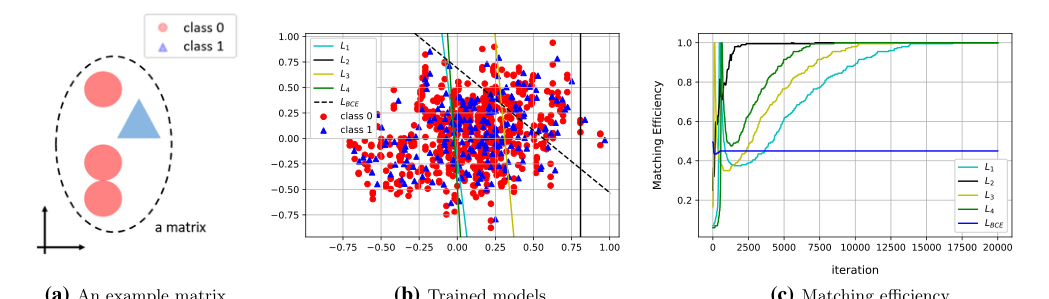 Figure 2. Experimental results from synthetic data. (a) An example matrix is illustrated. (b) The level sets of the trained models are drawn over the data scatter plot. (c) Matching efficiencies (evaluated on a test data set) for each of the loss functions are shown
This chosen method perfectly aligns with the harsh constraints of the problem. The ultimate goal is to maximize the matching efficiency, defined mathematically using the Kronecker delta function:
$$ \text{Matching efficiency} = \frac{1}{N} \sum_{i=1}^{N} \delta(y_i, \hat{y}(M_i)) $$
Because this step function is highly non-smooth and non-differentiable (returning zero gradients), it cannot be optimized directly via gradient descent. The "marriage" between the problem's constraints and the solution lies in the authors' clever design of surrogate loss functions. By treating the event matrix's row indices as distinctive categories, they transformed the problem into a multi-class classification or ranking task. For instance, their probabilistic ranking loss ($L_2$) and categorical cross-entropy loss ($L_3$) directly penalize the network if the true additional b-jet pair does not receive the highest relative score within its specific event strcuture.
To be honest, I'm not completely sure how trendy generative models like GANs, standard Diffusion, or Transformers would fare here, as the authors do not mention or imply them at all in the text. I suspect that applying a GAN or Diffusion model would be massive overkill and computationally wasteful for what is essentially a highly constrained combinatorial ranking problem. However, the authors explicitly explain the reasoning behind rejecting the most popular alternative—the binary classification DNN. They rejected it because optimizing $L_{BCE}$ mathematically misaligns with the physical objective. Even when they upgraded the binary classifier to include features from other b-jets in the event (their "Model 2"), it still fell short of their proposed surrogate losses ($L_2$ and $L_3$). The binary approach simply cannot guarantee that the highest-scoring pair in an event is actually correct, because it was never mathematically forced to compare them side-by-side during training.
Mathematical & Logical Mechanism
Imagine you are standing inside the control room of the Large Hadron Collider (LHC). Every time a colision happens, particles shatter at nearly the speed of light, creating showers of subatomic debris called "jets." Physicists are desperately hunting for the properties of the Higgs boson, which often decays into a specific type of debris called "b-jets."
However, there is a massive problem: a completely different, noisy background process called $t\bar{t}b\bar{b}$ (a top quark pair and a b quark pair) produces the exact same b-jets. To filter out this noise, physicists must figure out which b-jets came from the main event (top quark decays) and which were just extra debris (originating from a phenomenon called gluon splitting).
Previously, scientists used machine learning to look at every pair of b-jets in isolation, asking a simple yes/no question: "Are you the extra debris?" This binary classification approach was flawed because it ignored a fundamental rule of physics: in almost every valid event, there is exactly one pair of extra b-jets. By treating each pair independently, the old models were leaving valuable contextual information on the table.
The authors of this paper solved this by shifting the paradigm. Instead of asking "Is this pair the extra debris?", they designed a neural network to look at all the pairs in a single event simultaneously and ask, "Which of you is the most likely candidate?" They achieved this by abandoning standard binary accuarcy and designing custom loss functions to directly maximize "matching efficiency"—the rate at which the model picks the single correct pair out of the lineup.
Here is the absolute core mathematical engine that powers their most successful model, combining their event-level probability distribution (Softmax) with a Categorical Cross-Entropy surrogate loss:
$$ L_3 = -\frac{1}{N} \sum_{i=1}^N \log \left( \frac{\exp(g_{y_i}(M_i))}{\sum_{k=1}^{c_i} \exp(g_k(M_i))} \right) $$
Let's tear this equation apart piece by piece to understand how it works:
- $L_3$: This is the surrogate loss function. It acts as the ultimate error signal, telling the neural network how badly it messed up. The goal of the training process is to minimize this number.
- $-\frac{1}{N} \sum_{i=1}^N$: This calculates the average error across all $N$ events in the dataset. Why a summation and not an integral? Because the number of collision events $N$ is strictly discrete and countable. You cannot have a fraction of a collision, so integrating over a continuous space wouldn't make physical or logical sense here.
- $\log$: The natural logarithm. Its logical role is to heavily penalize the model when it is confidently wrong. If the model assigns a probability close to $1$ for the correct pair, the $\log$ of $1$ is $0$ (no penalty). But as the probability approaches $0$, the $\log$ plunges toward negative infinity, creating a massive rubber-band effect that violently pulls the model away from bad predictions.
- $M_i$: The $i$-th event matrix. This is the raw data input containing all the kinematic variables (like momentum and angles) for every b-jet pair in that specific collision.
- $y_i$: The index of the true additional b-jet pair in event $i$. It is the "ground truth" label provided by the physics simulation.
- $g_{y_i}(M_i)$: The neural network $g$'s raw output score (logit) for the correct b-jet pair. It acts as a raw confidence meter.
- $\exp(\dots)$: The exponential function. It serves two purposes: it ensures all scores are strictly positive, and it exaggerates the differences between high and low scores, making the network's preferences more decisive.
- $\sum_{k=1}^{c_i} \exp(g_k(M_i))$: The denominator sums the exponentiated scores of all $c_i$ possible b-jet pairs in event $i$. Why use addition instead of multiplication here? Addition pools the total "probability mass" of the event. If we multiplied them, we would be calculating the joint probability of independent events occurring simultaneously. But these pairs are mutually exclusive candidates for the single true signal, so we must add them to create a normalization factor.
- The fraction as a whole: This is the Softmax function. It takes the raw, unbounded scores and squashes them into a neat probability distribution that sums exactly to $1$.
Let's trace the exact lifecycle of a single abstract data point passing through this equation. Imagine an event matrix $M_i$ enters the assembly line containing three possible b-jet pairs.
First, the neural network processes the kinematic data of all three pairs and spits out raw scores: $2.0$ for the correct pair, and $0.5$ and $-1.0$ for the incorrect pairs.
Next, the $\exp$ function supercharges these scores, turning them into $7.39$, $1.65$, and $0.37$.
Then, the denominator gathers these values and adds them up to get a total pool of $9.41$.
The fraction then divides the correct pair's score by the total pool ($7.39 / 9.41$), resulting in a probability of roughly $0.78$.
Finally, the $\log$ function evaluates this $0.78$. Because it is relatively close to $1.0$, the resulting penalty is small. The data point has successfully passed through the engine.
How does this mechanism actually learn and converge? The optimization dynamics rely on the loss landscape created by the Softmax fraction. Because all the probabilities must sum to $1$, the model is forced into a zero-sum game. To minimize the loss, the network cannot just push the score of the correct pair up; it must simultaneously push the relative scores of the incorrect pairs down.
As the gradients flow backward through the network during training, they adjust the weights to recongize the subtle kinematic signatures (like angular distance and invariant mass) that distinguish gluon-splitting b-jets from top-quark b-jets. The loss landscape is shaped like a multi-dimensional valley where the lowest point corresponds to the network perfectly ranking the true b-jet pair above all others in every single event. To be honest, I'm not completely sure if the network architecture itself couldn't be further optimized with modern attention mechanisms, but the authors stuck to a standard feedforward design to brilliantly prove that simply fixing the mathematical objective function is enough to significantly outperform the old binary classification methods.
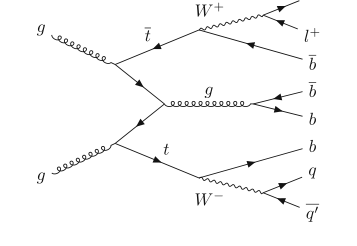 Figure 1. Feynman diagram of the t¯tb¯b process in the lepton+jets channel
Results, Limitations & Conclusion
The Grand Quest: Unmasking the Higgs Boson's Hiding Place
To understand the magnitude of this paper, we must first zoom out to the grandest stage of particle physics: the Large Hadron Collider (LHC). When physicists discovered the Higgs boson, it was a monumental triumph. But discovering it was only step one; step two is measuring its properties to ensure it behaves exactly as the Standard Model of particle physics predicts.
The Higgs boson loves to decay into a pair of bottom quarks ($b\bar{b}$). One of the best ways to study the Higgs is when it is produced alongside a top quark pair, a process known as $t\bar{t}H(b\bar{b})$. However, the universe is a messy place. There is a "background" process that looks almost exactly like our precious Higgs signal: the $t\bar{t}b\bar{b}$ process. This background process produces a top quark pair and a bottom quark pair, but without any Higgs boson involved. If we cannot perfectly understand and filter out this $t\bar{t}b\bar{b}$ background, our measurements of the Higgs boson will be forever blurred.
The Core Motivation and The Constraints
Here lies the fundemental problem: in a $t\bar{t}b\bar{b}$ event, you have $b$-jets (sprays of particles originating from bottom quarks) coming from two different sources. Some come from the decay of the top quarks, and some come from "gluon splitting" (where a gluon splits into two additional $b$-quarks). To understand the background, physicists desperately need to distingush the $b$-jets born from top quarks from the additional $b$-jets born from gluon splitting.
The Constraints:
1. Quantum Chaos: The kinematic properties (momentum, angles, energy) of these jets are governed by high-dimensional, stochastic quantum processes. There are no simple, hard-coded rules (like "if energy > X, then it's from a gluon") that work.
2. Combinatorial Explosions: An event doesn't just hand you two neat jets. It hands you a mess of particles. You have to look at pairs of jets and guess which pair is the "additional" one.
3. Overlapping Distributions: If you look at all $b$-jets across millions of events, the properties of top-decay jets and gluon-splitting jets overlap massively.
The Mathematical Interpretation: What Did They Solve?
The "Victim" (The Baseline Approach):
Previously, scientists treated this as a standard Binary Classification problem. They took every single pair of $b$-jets across all events, threw them into a Deep Neural Network (DNN), and asked: "Is this pair the additional $b$-jet pair? Yes (1) or No (0)?" They trained this using standard Binary Cross-Entropy ($L_{BCE}$):
$$ L_{BCE} = -\frac{1}{N_p} \sum_{i=1}^{N_p} \left( \xi_i \log f(x_i) + (1 - \xi_i) \log(1 - f(x_i)) \right) $$
The Flaw: This approach is mathematically blind to the structure of the data. It treats every pair in the universe as independent. But in reality, we know a crucial secret: Almost every single $t\bar{t}b\bar{b}$ event contains exactly ONE pair of additional $b$-jets.
The Brilliant Solution:
The authors realized that we shouldn't be asking "Is this pair an additional $b$-jet?" We should be looking at a single event and asking, "Out of all the pairs in this specific event, which one is the most likely to be the additional $b$-jet?"
They shifted the paradigm from global binary classification to event-level ranking (or multi-class classification within the event). They defined an event matrix $M_i \in \mathbb{R}^{c_i \times F}$, where $c_i$ is the number of $b$-jet pairs in the event, and $F$ is the feature dimension. They then applied a softmax function across the pairs within the event so their probabilities sum to 1:
$$ f_j(M_i) = \frac{\exp(g_j(M_i))}{\sum_{k=1}^{c_i} \exp(g_k(M_i))} $$
Because the ultimate goal is to maximize "matching efficiency" (the percentage of events where the correct pair is chosen), which is non-differentiable, they engineered four surrogate loss functions. The most conceptually beautiful is the probabilistic ranking loss ($L_2$), which forces the network to score the true additional pair higher than any other pair in that specific event:
$$ L_2 = -\frac{1}{N} \sum_{i=1}^N \sum_{j \neq y_i} \log \left( \frac{f_{y_i}(M_i)}{f_{y_i}(M_i) + f_j(M_i)} \right) $$
They also utilized a categorical cross-entropy loss ($L_3$) treating the correct pair index as the true class:
$$ L_3 = -\frac{1}{N} \sum_{i=1}^N \log f_{y_i}(M_i) $$
Ruthless Experimental Architecture and Definitive Evidence
The authors didn't just throw metrics at the wall; they architected a two-stage execution to ruthlessly prove their mathematical claims.
Stage 1: The Synthetic Trap (Proof of Concept)
They first built a 2D synthetic dataset designed to perfectly mimic the overlapping nature of the physics data. They created events where the "signal" and "background" overlapped globally but were distinct locally within an event. The binary classifier (the victim) failed miserably, drawing an arbitrary decision boundary because it was confused by the global overlap. The authors' new loss functions achieved a 100% matching efficiency because they only compared points within their respective events. It was a flawless mathematical checkmate.
Stage 2: The LHC Simulation
They then simulated actual proton-proton collisions at $\sqrt{s} = 13$ TeV using a heavy-duty physics pipeline: MadGraph5_aMC@NLO (event generation) $\rightarrow$ Pythia (hadronization) $\rightarrow$ DELPHES (CMS detector simulation). This is as close to real LHC data as you can get without spending \$150 million on collider time.
The Definitive Evidence:
They didn't just say "accuracy improved." They proved that by changing only the loss function to respect the event structure, the matching efficiency improved undeniably. For the Leading Order (LO) simulations, efficiency jumped from 62.1% (using the $L_{BCE}$ victim model) to 64.5% (using their $L_3$ model).
But the most undeniable evidence is visual and physical: Figure 3. They plotted the reconstructed physical distributions—specifically the angular distance ($\Delta R$) and the invariant mass of the $b$-jet pairs. The histograms generated by their proposed method hugged the "True Signal" (generator-level truth) significantly tighter than the binary classification approach. They proved that their AI wasn't just learning statistical noise; it was recovering the underlying quantum kinematics more accurately.
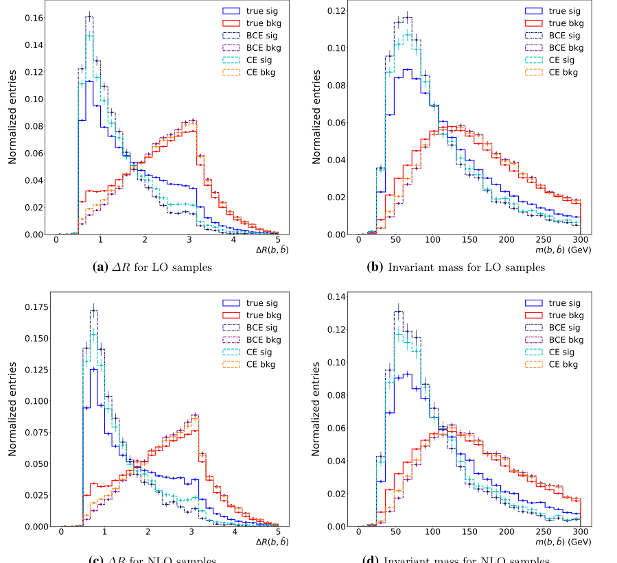 Figure 3. Reconstructed-level distributions of ?R (angular distance) and invariant mass of b-jet pairs in the test sets of LO samples (for (a) and (b)) and NLO samples (for (c) and (d)). The additional b-jet pairs are denoted the signal (sig), and the other b-jet pairs are denoted the background (bkg). Additional b-jet pairs are identified according to three different criteria (true: matched to the generator-level information at the LO or NLO, BCE: the prediction from the binary classification approach, CE: the prediction from our method using L3, i.e., the cross-entropy loss)
Future Discussion Topics for the Brilliant Mind
Based on this paper, here are several avenues we must explore to push this frontier further:
-
Beyond Feedforward Networks: The Era of Graph Neural Networks (GNNs)
The authors used a Deep Feedforward Neural Network that processes pairs and then aggregates them. However, an event is inherently a graph of interacting particles. How much more matching efficiency could we achive if we modeled the entire event as a fully connected graph using Attention mechanisms or GNNs, allowing the network to learn the relational physics between all jets simultaneously? -
End-to-End Raw Detector Learning
Currently, this method relies on 78 pre-calculated kinematic variables (like transverse momentum, pseudorapidity). What if we bypassed human-engineered features entirely? Could we feed the raw 3D point-cloud data from the CMS detector's particle-flow algorithm directly into a 3D Convolutional or PointNet architecture to let the AI discover kinematic invariants we haven't even thought of? -
Domain Adaptation for Real Collision Data
This paper relies heavily on Monte Carlo simulations (MadGraph/Pythia). However, simulations are never perfect replicas of real LHC data. How can we integrate unsupervised domain adaptation techniques (like Gradient Reversal Layers) to ensure that the matching efficiency gains observed in this simulated environment transfer flawlessly to the actual, messy data of the upcoming High Luminosity LHC (HL-LHC) runs?