Counterfactual Explanations for Conformal Prediction Sets
New counterfactual explanations make complex "prediction sets" from AI understandable by showing minimal changes that alter the AI's output.
Background & Academic Lineage
Machine learning models are increasingly deployed in high-stakes environments—such as medical diagnoses or financial loan approvals—where a \$150 mistake might be a minor inconvenience, but a \$150,000 mistake could be catastrophic. In these critical domains, simply providing a single "best guess" (a point prediction) is not enough. Decision-makers need to understand the model's uncertainty.
To solve this, the academic field developed Conformal Prediction (CP) around 2005. Instead of outputting a single label, a conformal predictor outputs a set of plausible labels with a mathematical gaurantee that the true label is included (e.g., "I am 95% sure the patient's condition is either Healthy or Diabetic").
Simultaneously, as machine learning models became complex "black boxes," the field of Explainable AI (XAI) emerged. One of the most intuitive XAI techniques is the Counterfactual Explanation (popularized around 2017), which tells a user exactly what minimal changes are needed to flip a model's decision.
The specific problem addressed in this paper emerged at the exact intersection of these two fields: How do we explain the uncertainty-aware sets produced by conformal predictors? While we have great tools to explain single predictions, and great tools to quantify uncertainty, we lacked a bridge to explain why a model's uncertainty shifted enough to include or exclude a specific label in a prediction set.
The fundamental limitation—or "pain point"—of previous approaches is that existing counterfactual explanation methods were strictly designed for point predictors. They assume the model outputs exactly one label, and their entire mathematical objective is to find the smallest feature tweak to flip that one label to another.
Because conformal predictors output sets of labels (which expand or shrink based on the model's confidence), existing methods completely fall short. They specifcally cannot explain changes in prediction set outputs. For example, older methods cannot answer: "What small change in this patient's blood pressure would make the model confident enough to drop 'Diabetic' from the realm of possibility?" Furthermore, while a few recent models tried to incorporate uncertainty into counterfactuals, they lacked formal, distribution-free statistical guarantees. The authors were forced to write this paper to invent a new type of counterfactual that targets the inclusion or exclusion of labels within a guaranteed prediction set.
Here are a few highly specialized terms from the paper, translated into everyday concepts:
- Conformal Prediction Set:
- Analogy: Imagine fishing. A standard model uses a spear (a point prediction)—it aims for exactly one fish, but if it misses, you get nothing. A conformal predictor uses a net (a prediction set). The net might catch a little seaweed along with the fish, but it guarantees you will catch the fish 95% of the time. The size of the net represents uncertainty: a small net means high certainty, while a massive net means the model is very unsure.
- Counterfactual Explanation:
- Analogy: A GPS rerouting suggestion. Instead of just telling you "You are stuck in traffic" (a standard prediction), a counterfactual explanation tells you, "If you had taken the previous exit, you would be driving at the speed limit right now." It shows the minimal change required to get a different outcome.
- Credibility:
- Analogy: A bouncer at an exclusive club checking your vibe. In this paper, credibility measures how well a new, synthetic data point (the counterfactual) blends in with the real data the model was trained on. If credibility is high, the new data point looks like a normal, plausible person. If it's low, the data point is an unrealistic alien that the model has never seen before.
- Sparsity:
- Analogy: A mechanic fixing your car. You want them to replace just the one broken spark plug (high sparsity) rather than rebuilding the entire engine and changing the tires (low sparsity). In the paper, a sparse explanation changes as few variables as possible, making it easier for a human to understand and act upon.
| Notation | Description |
|---|---|
| $x$ | The original input instance (the test data point) that needs to be explained. |
| $x'$ | The surrogate counterfactual instance; the newly generated data point that changes the prediction set. |
| $x^{\text{real}}$ | A real counterfactual instance found within the calibration dataset, used to anchor the search space. |
| $\epsilon$ | The predefined significance level (e.g., $0.05$), representing the acceptable error rate. |
| $\mathcal{Y}$ | The set of all possible class labels in the dataset. |
| $\tilde{y}$ | A candidate label being tested for inclusion in the prediction set. |
| $\Gamma^\epsilon(x)$ | The conformal prediction set for instance $x$ at significance level $\epsilon$. It contains all labels that were not rejected. |
| $Z^c$ | The calibration dataset, a separate set of data used to compute nonconformity scores. |
| $p_k(x)$ | The p-value computed by the conformal predictor for class $k$ at instance $x$. |
| $h$ | The underlying machine learning algoritm/classifier used to make the base predictions. |
| $\alpha_i$ | The nonconformity score, measuring how "strange" an instance is compared to known data. |
| $d(x, c)$ | A distance metric (like Euclidean or Gower distance) measuring how far the counterfactual $c$ is from the original input $x$. |
Problem Definition & Constraints
Imagine you are using an AI to help diagnose a patient. A traditional AI model gives you a single, confident guess: "This patient has diabetes." But in high-stakes fields like medicine or finance, a single guess isn't enough; we need to know when the model is uncertain. Enter conformal prediction. Instead of a single label, a conformal classifier outputs a prediction set—a list of plausible labels (e.g., {Healthy, Diabetic}) with a mathematical gaurantee that the true answer is inside that set, say, 95% of the time. If the AI is highly uncertain, the set gets larger; if it is certain, the set shrinks to a single label.
But here is where we hit a wall: how do we explain why the AI gave us this specific set? For traditional AI, we use "counterfactual explanations." These are "what-if" scenarios, such as: "If this patient's BMI was 2 points lower, the AI would have predicted 'Healthy' instead of 'Diabetic'."
The starting point (Input/Current State) of this paper is the existence of these conformal prediction sets and traditional counterfactual methods. However, traditional counterfactuals are strictly designed to flip a single point prediction. The desired endpoint (Output/Goal State) is a brand-new type of explanation: a conformal counterfactual. The authors want to find the minimal changes to a test instance that will alter the entire prediction set at a fixed confidence level—for example, figuring out exactly what needs to change to drop "Diabetic" from the set of possibilities entirely.
The mathematical gap this paper bridges lies in the optimization objective. Traditional counterfactuals solve a problem that looks like this:
$$ \min_{c \in \mathcal{X}} d(x, c) \quad \text{subject to} \quad f(x) \neq f(c) $$
Here, you want to find a new instance $c$ that minimizes the distance $d$ from the original input $x$, as long as the predicive model $f$ outputs a different single label.
The authors had to rewrite this logic for sets. Instead of a single label $f(x)$, they are dealing with a prediction set $\Gamma^\epsilon(x)$ at a significance level $\epsilon$. Their new objective requires finding a surrogate instance $x'$ such that the set itself changes:
$$ \Gamma^\epsilon(x') \neq \Gamma^\epsilon(x) $$
Furthermore, they introduced a novel metric called credibility to guide this search. Credibility is defined mathematically as the maximum p-value across all candidate classes $k$:
$$ \text{Credibility}(x') = \max_k p_k(x') $$
This measures how well the new "what-if" scenario actually conforms to the underlying distribution of the real training data.
However, in the world of explainable AI, fixing one thing almost always breaks another. The painful dilemma trapping previous researchers is the tug-of-war between Proximity/Sparsity and Plausibility.
If you simply ask an algoritm to find the mathematically shortest distance to change a prediction (Proximity), or to change the fewest number of features (Sparsity), the math will happily oblige by creating a Frankenstein data point. It might tell you, "To get an income over \$50,000, simply change your age to 150 years old." It is mathematically close, but physically impossible. Previous researchers struggled to generate counterfactuals that were minimal but still resided on the true "data manifold" (meaning they look like realistic, plausible human beings or scenarios).
To solve this, the authors slammed into several harsh, realistic walls:
- The Infinite Search Space Constraint: You cannot just search every possible combination of numbers to find a counterfactual. The continuous feature space is infinitely large. To overcome this, the authors had to strictly bound the search. They first find a "real counterfactual" $x^{\text{real}}$—an actual, historical data point from a calibration dataset that yields a different prediction set. They then build a discrete grid of feature values strictly bounded between the original instance $x$ and $x^{\text{real}}$.
- Combinatorial Explosion: Even after restricting the search to this bounded grid, the number of possible feature combinations grows exponentially. If a dataset has many features, checking every combination is computationally impossible. The authors hit a hard computational limit: if the number of combinations exceeds 10,000, exhaustive search crashes or takes too long. They were forced to abandon perfect optimization and rely on a heuristic Genetic Algorithm to navigate the space.
- The Burden of Conformal Computation: Unlike simple neural networks where a forward pass is lightning fast, conformal prediction requires calculating nonconformity scores and p-values for every single candidate label for every single synthetic data point generated during the search. This creates a massive computational bottleneck, making real-time generation of these explanations incredibly difficult.
Why This Approach
To truly understand the breakthrough in this paper, we first need to look at how traditional AI makes decisions. Most machine learning models are "point predictors"—they look at your data and give you a single, absolute answer, like "This patient is Diabetic." But in high-stakes fields like medicine or finance, a single guess isn't enough; decision-makers need to know the model's uncertainty. This is where Conformal Prediction (CP) comes in. Instead of a single label, CP outputs a prediction set (e.g., $\{\text{Healthy}, \text{Diabetic}\}$) with a mathematical guarantee that the true answer is inside that set with a specific probability, say $95\%$.
The authors reallized that traditional state-of-the-art (SOTA) explanation methods were fundamentally broken for these uncertainty-aware models. Standard counterfactual methods are designed exclusively for point predictors. They answer the question: "What is the minimal change needed to flip the model's prediction from A to B?" However, when your model outputs a set of plausible labels rather than a single label, existing methods completely fall apart. You cannot simply "flip" a set. The exact moment of realization came when the authors saw that to explain model uncertainty, they needed to explain why a specific class was included or excluded from the prediction set at a fixed significance level $\epsilon$. A completely new mathematical framework tailored to conformal prediction was the only viable solution.
Beyond simple performance metrics, this method is qualitatively superior because of its structual advantage in handling plausibility. The previous gold standard for counterfactuals relied heavily on minimizing distance (like the $\ell_2$ norm) or sparsity (the number of changed features). While this works mathematically, it often generates "alien" data points—suggestions that look nothing like real-world instances. To solve this, the authors introduced a groundbreaking metric: credibility.
In conformal prediction, credibility is defined as the maximum p-value across all candidate labels:
$$ \text{Credibility}(x') = \max_k p_k(x') $$
By optimizing for credibility, the method ensures that the generated counterfactual $x'$ perfectly conforms to the underlying training data distribution. Instead of forcing a massive, unrealistic leap across a decision boundary to change a point prediction, this method finds smaller, highly plausible nudges that simply expand or shrink the uncertainty set. For example, in the Income dataset, shifting a prediction set from $\{>\$50\text{K}, \leq\$50\text{K}\}$ to a more confident singleton set $\{>\$50\text{K}\}$ requires much more realistic feature changes than forcing a rigid class flip.
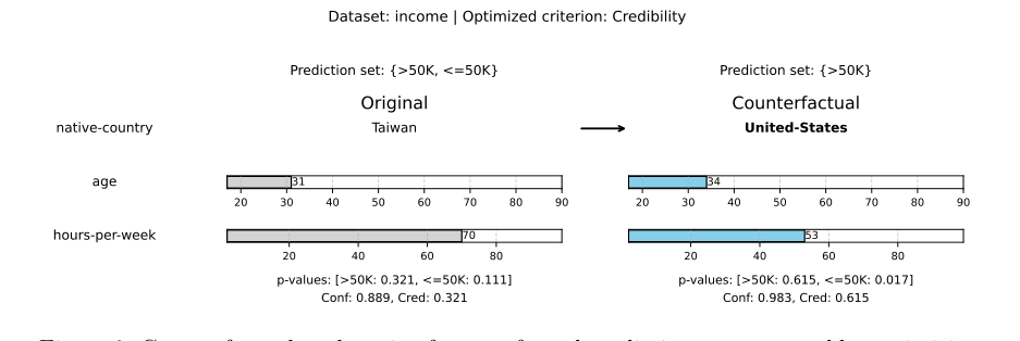 Figure 6. Counterfactual explanation for a conformal prediction set generated by optimizing for credibility on the income dataset. Only changed features are shown
The problem presented harsh constraints: the explanations had to be mathematically valid under the conformal framework, actionable, and strictly tied to the calibration data to maintain distribution-free guarantees. The chosen appraoch perfectly marries these constraints. The authors designed a discrete search space bounded by the original test instance $x$ and the closest real counterfactual $x^{\text{real}}$ found in the calibration set $Z^c$:
$$ x^{\text{real}} = \arg \min_{x_i \in Z^c} \{ \| x - x_i \|_2 \mid \Gamma^\epsilon(x_i) \neq \Gamma^\epsilon(x) \} $$
By anchoring the search space to actual observed values, the algorithm guarantees that the synthetic counterfactual never strays into impossible feature combinations. If the search space is small, it uses an exhaustive search; if it becomes computationally massive, it elegantly scales using a Genetic Algorithm. This is a perfect marriage: the rigorous statistical bounds of conformal prediction are maintained while providing intuitive, human-readable explanations.
Finally, the paper explicitly points out why other popular approaches would have failed here. Recent attempts to incorporate uncertainty into counterfactuals using Bayesian modeling or epistemic uncertainty quantification completely miss the mark for this specific problem. Bayesian models provide probabilistic scores, but they lack distribution-free guarantees. They assume a prior distribution, and if that assumption is wrong, the guarantees collapse. Conformal prediction relies only on the assumption of exchangeability. Therefore, trying to shoehorn Bayesian counterfactuals or standard generative models (like GANs or Diffusion) into this pipeline would destroy the strict, mathematically proven error rate that makes conformal prediction so valuable in the first place. The authors had to reject those alternatives to preserve the absolute statistical validity of the prediction sets.
Mathematical & Logical Mechanism
To understand the breakthrough in this paper, we first need to establish a baseline of how modern AI makes decisions and how we measure its uncertainty.
In traditional machine learning, a model gives you a "point prediction"—a single, best-guess answer. However, in high-stakes fields like medicine or finance, a single guess isn't enough; we need to know how confident the model is. Enter Conformal Prediction (CP). Instead of a single answer, CP outputs a prediction set with a mathematical guarantee. For example, it might say, "I am 95% confident that this patient's diagnosis is either {Healthy, Diabetic}." If the model is highly uncertain, the set grows larger. If it is certain, the set shrinks to a single label.
The motivation behind this paper stems from a critical blind spot in Explainable AI. When an AI makes a point prediction, we often use counterfactual explanations to understand it ("If your income was higher, your loan would have been approved"). But how do you explain a prediction set? Existing methods completely fail here. The authors set out to solve this by finding the minimal changes required to alter the model's uncertainty boundry, effectively explaining why certain classes were included or excluded from the set.
To do this, they had to overcome several constraints: the generated explanation must be close to the original data (Proximity), it must change as few variables as possible (Sparsity), and crucially, it must actually look like a realistic data point rather than a mathematical hallucination (Credibility).
Here is the mathematical engine they built to solve this.
The Master Equations
The core logic of this paper is driven by a three-part mathematical engine: finding a reality anchor, maximizing plausibility, and penalizing complexity.
$$ x^{\text{real}} = \arg \min_{x_i \in Z^c} \left\{ \|x - x_i\|_2 \mid \Gamma^\epsilon(x_i) \neq \Gamma^\epsilon(x) \right\} $$
$$ \text{Credibility}(x') = \max_k p_k(x') $$
$$ \text{Sparsity}(x, x') = \sum_{j=1}^p \mathbf{1}\{x_j \neq x'_j\} $$
Tearing the Equations Apart
Let's break down every single component of this engine to understand its physical and logical role.
- $x$: The original input data point (e.g., a patient's current health metrics). This is our starting line.
- $x_i \in Z^c$: A real data point from the calibration dataset $Z^c$. Its logical role is to act as a "reality check" so the model doesn't invent impossible scenarios.
- $\|x - x_i\|_2$: The L2 norm (Euclidean distance). This acts as a rubber band pulling the search back toward the original input. The authors use the L2 norm here because it heavily penalizes large, unrealistic deviations in any single variable, forcing the model to find a balanced, nearby solution.
- $\Gamma^\epsilon(x)$: The conformal prediction set at a fixed significance level $\epsilon$ (usually 0.05 for 95% confidence). This represents the boundry of the model's uncertainty.
- $\neq$: The inequality operator. This is the logical trigger of the entire paper. We don't just want to shift underlying probabilities; we demand a structural, visible change in the final prediction set.
- $\arg \min$: The search operator. It scans the data to find the path of least resistance—the absolute closest real-world example that successfully flips the prediction set.
- $x'$: The synthetic surrogate counterfactual we are generating. This is the final explanation we will hand to the user.
- $p_k(x')$: The p-value for class $k$. In conformal prediction, this measures how well the new point conforms to the known data distribution for that specific class.
- $\max_k$: The maximum operator. By taking the maximum p-value across all classes, it ensures the counterfactual is highly plausible for at least one class, rather than averaging out to a mediocre, unrealistic state.
- $\sum_{j=1}^p$: The summation over all $p$ features. Why did the authors use a summation instead of a product here? Because we want to count the total number of altered features additively. If we used multiplication, a single unchanged feature (yielding a 0) would wipe out the entire penalty, completely breaking the logic of counting changes.
- $\mathbf{1}\{x_j \neq x'_j\}$: The indicator function. It acts as a binary switch: it outputs $1$ if a feauture was changed, and $0$ if it was left alone.
Step-by-step Flow
Let's trace a single abstract data point as it moves through this mechanical assembly line:
- The Input: A patient's data $x$ enters the system. The model is uncertain and outputs a prediction set of {Healthy, Diabetic}.
- The Reality Anchor: The system scans the historical calibration data to find $x^{\text{real}}$, the closest actual patient who received a different prediction set (e.g., just {Healthy}).
- The Grid Construction: A discrete search grid is built. The system extracts all observed values between $x$ and $x^{\text{real}}$. This ensures we only suggest realistic intermediate steps (e.g., we won't suggest a blood pressure of 10 if it doesn't exist in the data).
- The Assembly Line: A synthetic candidate $x'$ is generated on this grid. It passes through the conformal predictor to see if its prediction set actually flips ($\Gamma^\epsilon(x') \neq \Gamma^\epsilon(x)$).
- Quality Control: If the set flips, the candidate is evaluated. The system calculates its Credibility (is it a realistic patient?) and its Sparsity (did we only change a few things, like just 'Glucose' and 'Age'?).
- The Output: The candidate that best balances these criteria is returned as the final, actionable explanation.
Optimization Dynamics
How does this mechanism actually learn, update, and converge?
In traditional neural networks, we use gradient descent to slide down a smooth loss landscape. However, because conformal prediction sets create hard, non-differentiable step-functions (a label is either strictly inside the set or outside of it), gradients do not exist here. The loss landscape isn't a smooth hill; it's a jagged cliff face of discrete, binary decisions.
To overcome this, the authors use a two-pronged optimzation strategy. If the search space is small (under 10,000 combinations), the system uses a brute-force exhaustive search, evaluating every single point on the grid to find the absolute mathematical optimum.
If the space is too large, it deploys a Genetic Algorithm (GA). The GA initializes a population of 100 random candidate counterfactuals. The "fitness" of each candidate is determined by our Master Equations (maximizing Credibility or minimizing Sparsity). Crucially, the landscape is shaped by a massive penalty function: if a candidate fails to change the prediction set, its fitness score is destroyed, effectively killing it off in the next generation. Over 1,000 iterations, candidates mutate (randomly tweaking a feature by a 10% probability) and crossover (swapping features between two good candidates).
To be honest, I'm not completely sure why the authors hardcoded the genetic algorithm's elitism ratio exactly at 0.01 without an ablation study, but in practice, it is just enough to keep the absolute best candidate alive across generations without stalling the search. Through this evolutionary process, the system iteratively converges toward a minimal, highly credible change that successfully alters the model's uncertainty boundary.
Results, Limitations & Conclusion
Imagine you go to a doctor for a medical diagnosis. If the doctor says, "You definitely have diabetes," that is a standard point prediction. But what if the doctor says, "Based on your tests, I am 95% sure you are either completely healthy or you have early-stage diabetes"? This second scenario is the essence of Conformal Prediction (CP). Instead of giving a single, potentially overconfident answer, CP gives you a prediction set—a list of possible outcomes backed by a mathematical guarentee that the true answer is inside that set with a specific probability.
However, this introduces a massive psychological and practical problem: Why did the model include "diabetes" in that set? What would need to change about your health profile for the model to confidently drop "diabetes" and just say "healthy"?
This is where Counterfactual (CF) Explanations come in. A counterfactual is a "what-if" scenario. It tells you the minimal change required to alter a model's decision (e.g., "If your blood pressure was 10 points lower, you would be classified as strictly healthy"). Historically, scientists have only figured out how to generate counterfactuals for standard point predictions. This paper tackles a brilliant, previously unsolved problem: How do we generate counterfactual explanations for conformal prediction sets?
The Background and Motivation
To understnad this paper, you need to grasp two concepts:
1. Conformal Prediction Sets: Given a significance level $\epsilon$ (say, 0.05 for a 95% confidence level), a conformal classifier outputs a set of labels $\Gamma^\epsilon(x)$. It does this by calculating a nonconformity score for every possible label, converting those into $p$-values, and rejecting any label where the $p$-value is less than $\epsilon$.
2. Counterfactuals: These are synthetic data points $x'$ that are very close to the original input $x$, but result in a different prediction.
The motivation here is pure trust and actionability. Decision-makers don't just want to know the uncertainty of a model; they want to know the boundaries of that uncertainty. If a bank's model says your loan application prediction set is $\{\text{Approved}, \text{Denied}\}$, you want to know exactly what to change (e.g., paying off \$150 in credit card debt) to shift that set to strictly $\{\text{Approved}\}$.
The Constraints to Overcome
Generating these "what-if" scenarios is incredibly difficult due to the vastness of high-dimensional data. If you just let an algorithm blindly search for a mathematical solution, it will suggest absurd things, like "decrease your age by 15 years" or "have a negative blood pressure."
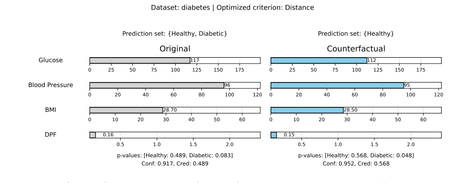 Figure 1. Counterfactual explanation for a conformal prediction set generated by optimizing for distance on the Diabetes dataset. Only changed features are shown
Therefore, the authors had to constrain the search space so the generated explanations are:
* Proximate: The change must be small.
* Sparse: It should only change one or two features, not all of them.
* Plausible (Credible): The synthetic data point must look like real data from the real world.
The Mathematical Problem and Solution
The core mathematical problem the authors solved is finding a surrogate instance $x'$ such that the prediction set changes:
$$ \Gamma^\epsilon(x') \neq \Gamma^\epsilon(x) $$
To solve this without generating impossible data points, they engineered a highly constrained, three-step search architecure:
1. Find a "Real" Counterfactual: First, they look at the calibration dataset (real historical data) and find the closest actual data point $x^{\text{real}}$ that has a different prediction set than $x$.
2. Build a Grid: They construct a discrete search space bounded entirely by the values between $x$ and $x^{\text{real}}$. This guarantees the algorithm can't invent wild, out-of-bounds numbers.
3. Optimize: They search this grid (using exhaustive search for small spaces, or a Genetic Algorithm for larger ones) to find a synthetic $x'$ that optimizes one of three criteria:
* Distance (Proximity): Minimizing $||x - x'||_2$.
* Sparsity: Minimizing the number of changed features $\sum_{j=1}^p \mathbf{1}\{x_j \neq x'_j\}$.
* Credibility: This is the authors' masterstroke. They define credibility as $\max_k p_k(x')$. By maximizing the highest $p$-value across all classes, they force the counterfactual to conform tightly to the underlying distribution of the training data. It mathematically forces the "what-if" scenario to be highly realistic.
The Experimental Architecture and the "Victims"
The authors didn't just list metrics; they designed a ruthless experiment to prove their synthetic counterfactuals were better than reality itself.
The "Victims": Because no other algorithm exists to generate counterfactuals for conformal prediction sets, the baselines (the "victims" they had to defeat) were the real counterfactuals ($x^{\text{real}}$) pulled directly from the historical dataset.
The Evidence: They tested their method across 10 tabular datasets. For each dataset, they generated surrogate counterfactuals and compared them to the real counterfactuals using a ratio.
* When optimizing for distance, their method achieved an average ratio of $0.452$. This is undeniable evidence that their algorithm found valid explanations that were 54.8% closer to the original input than the best real-world example.
* When optimizing for sparsity, they achieved a ratio of $0.493$, meaning their explanations required changing half as many features as the real-world counterparts.
* Most impressively, when optimizing for credibility, they achieved a ratio of $1.157$. This means their synthetic, mathematically generated data points were actually 15.7% more conforming to the data distribution than actual, real data points from the calibration set.
To be honest, I'm not completely sure why they settled on a relatively basic Genetic Algorithm package for the larger search spaces when more advanced discrete gradient-based optimizers exist, but the empirical evidence proves it was more than sufficient as a proof-of-concept.
Discussion Topics for Future Evolution
Based on this brilliant foundation, here are several critical avenues for future research:
- Causal Graphs and Strict Actionability: The current method bounds the search space using real data, but it doesn't understand causality. In their diabetes example, the algorithm suggested decreasing a patient's age from 30 to 26. Age is immutable.
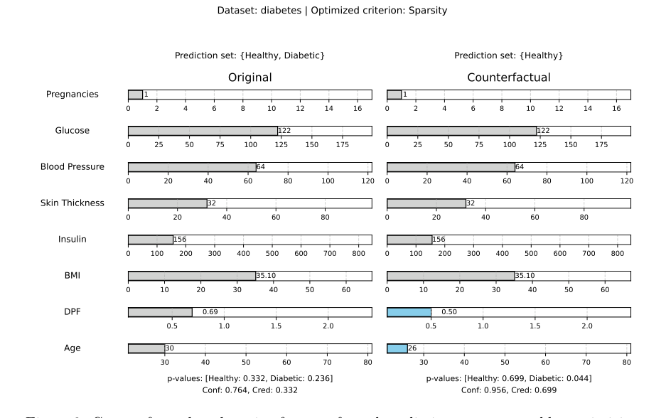 Figure 3. Counterfactual explanation for a conformal prediction set generated by optimizing for sparsity on the Diabetes dataset. Changed features are shown in blue
How can we integrate Directed Acyclic Graphs (DAGs) into the conformal search space so that the algorithm only suggests causally downstream, actionable interventions?
2. Targeted Set Steering: Currently, the algorithm stops as soon as the prediction set changes ($\Gamma^\epsilon(x') \neq \Gamma^\epsilon(x)$). But what if the user wants to steer the set in a specific direction? For example, moving from $\{\text{Benign}, \text{Malignant}\}$ strictly to $\{\text{Benign}\}$. How can we modify the objective function to target specific set inclusions/exclusions?
3. Scaling to Unstructured Data: This method relies on a discrete grid search between tabular features. How do we evolve this to work with high-dimensional unstructured data, like images or text? Could we map the conformal $p$-values to a continuous latent space in a Variational Autoencoder (VAE) and perform gradient descent to find the counterfactual image?
4. Balancing the Trilemma: The authors optimized for distance, sparsity, and credibility separately. Can we formulate a Pareto-optimal loss function that balances all three simultaneously, perhaps using multi-objective reinforcement learning, to find the ultimate "perfect" explanation?
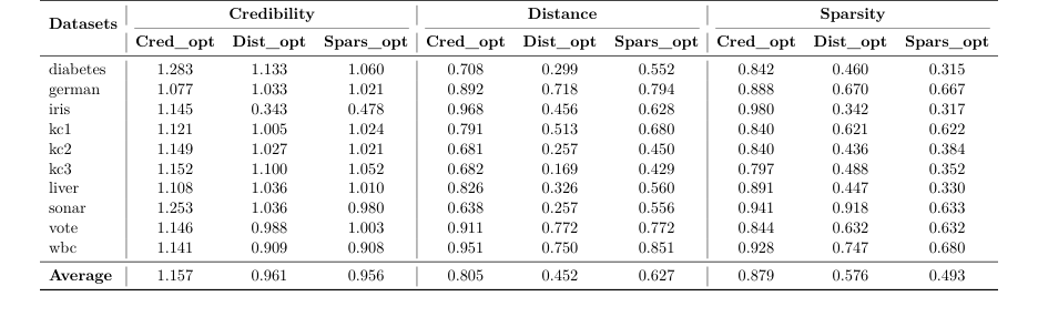 Table 2. Comparison of optimization criteria across datasets