Anatomical Structure Few-Shot Detection Utilizing Enhanced Human Anatomy Knowledge in Ultrasound Images
Deep learning-based models have significantly advanced clinical ultrasound tasks by detecting anatomical structures within vast ultrasound image datasets.
Background & Academic Lineage
The field of medcial image analysis has experienced massive leaps forward thanks to deep learning. However, the specific problem addressed in this paper stems from a severe, real-world bottleneck: data hunger. Traditionally, training an AI to detect fetal organs in ultrasound images requires vast datasets. These datasets must be meticulously annotated by highly specialized doctors, a process that is incredibly tedious and expensive (often costing well over \$150 per hour in expert labor). Furthermore, strict ethical and privacy regulations make gathering and sharing large-scale patient data nearly impossible.
To bypass this data scarcity, the academic field pivoted to "few-shot learning"—a paradigm designed to train models using only a tiny handful of examples. While few-shot learning has seen great success in basic tasks like classifying an entire image or outlining a single organ (semantic segmentation), it historically ignored the much more complex task of multi-object detection in ultrasound images. The authors recognized this gap and initiated this research to bring few-shot detection to complex, multi-organ ultrasound environments.
The authors were forced to write this paper because previous approaches hit two fundamental limitations:
1. Vulnerability to Domain Shifts: Ultrasound images are notoriously messy. They suffer from severe variations depending on the machine's brand, the operator's probe angle, and inherent speckle noise. Previous few-shot models failed to generalize across these variations because they lacked a unified understanding of human anatomy to anchor their predictions.
2. Architectural Blind Spots in Modern Sequence Models: Recently, a highly efficient AI architecture called "Mamba" (based on State Space Models) became popular for processing long sequences of data. However, previous Mamba-based methods only focused on spatial correlations and completely neglected "channel information" (the deep, layered feature representations). This lack of channel mixing caused stability issues in larger networks and severely limited the model's ability to understand the global context of the anatomical structurs.
To make the highly specialized concepts in this paper intuitive, here are four key domain terms translated into everyday analogies:
- Few-Shot Learning: Imagine teaching a child what a "platypus" is. You don't need to show them 10,000 pictures; just three or four good photos are enough for them to recognize one in the wild. Few-shot learning tries to give AI this same human-like ability to learn from very limited examples, instead of relyng on massive datasets.
- Domain Shift: Think of listening to your favorite song played on a cheap, static-filled radio versus a high-end concert sound system. The underlying song is exactly the same, but the audio quality and distortion vary wildly. In ultrasounds, different machines and doctors create a "domain shift" that easily confuses standard AI models.
- Topological Relationship Reasoning (TRR): Imagine trying to put together a jigsaw puzzle in a dimly lit room. Even if you can't see the pieces clearly, you know logically that the "chimney" piece must connect to the "roof" piece. TRR gives the AI a similar logical map: it uses the fixed, natural layout of human organs (e.g., the heart is always near the lungs) to find structures even when the ultrasound image is blurry.
- Selective State Space Models (SSMs): Picture a busy lawyer reading a 500-page legal document. Instead of memorizing every single word, they selectively highlight only the critical clauses and ignore the useless filler text. SSMs do this for data, dynamically filtering out irrelevant noise to process information incredibly fast and efficiently.
Here is a breakdown of the key mathematical notations used to formulate the authors' solution:
| Notation | Type | Description |
|---|---|---|
| $x(t), y(t)$ | Variable | One-dimensional input and output sequences processed by the State Space Model. |
| $h(t)$ | Variable | The hidden state that maps the input sequence to the output sequence. |
| $A, B$ | Parameter | Continuous-time parameters that govern the linear time-invariant system. |
| $\overline{A}, \overline{B}$ | Parameter | Discrete-time parameters converted from their continuous counterparts for computation. |
| $\Delta$ | Parameter | A timescale parameter used to discretize the continuous parameters. |
| $X$ | Variable | The input tensor representing the image features, defined as $X \in \mathbb{R}^{B \times C \times H \times W}$. |
| $B, C, H, W$ | Parameter | Dimensions of the feature map: Batch size, number of Channels, Height, and Width. |
| $G = \langle \mathcal{N}, \mathcal{E} \rangle$ | Variable | An undirected region-to-region graph where nodes $\mathcal{N}$ are region proposals and edges $\mathcal{E}$ are relationships. |
| $z_i$ | Variable | The latent space representation of visual features for a specific node $i$. |
| $\omega_m(P(i, j))$ | Variable | A Gaussian kernel function that encodes the spatial distance and angle between two anatomical regions. |
Problem Definition & Constraints
Imagine trying to find a specific set of keys in a dark, foggy room. Now imagine you’ve only been shown what those keys look like three or five times in your entire life. This is essentially the challenge of few-shot object detection in medical ultrasound imaging.
To understand the magnitude of the problem this paper tackles, we first need to define exactly where we are starting, where we want to go, and why the journey between those two points is so treacherous.
The Starting Point and The Goal State
The Input (Current State): The system is fed a raw, highly noisy ultrasound image—specifically fetal ultrasound scans (like the brain or heart). Alongside this, the model is given an extremely limited set of annotated examples (as few as 1, 3, 5, or 10 "shots") of novel anatomical structures it needs to learn. Mathematically, the input is a high-dimensional visual feature tensor $X \in \mathbb{R}^{B \times C \times H \times W}$, where $B$ is the batch size, $C$ is the number of channels, and $H$ and $W$ are the spatial dimensions.
The Output (Goal State): The model must output precise bounding boxes and classification scores for multiple anatomical structures within that blurry image. This is represented as a regional prediction matrix $S \in \mathbb{R}^{N \times C}$, where $N$ is the number of region proposals and $C$ is the number of classes.
The Mathematical Gap: The missing link is a robust mapping function that can bridge $X$ to $S$ without overfitting to the tiny training dataset. Standard deep learning models map this space by relyng on millions of parameter updates driven by massive datasets. In a few-shot scenario, the mathematical space is severely under-constrained. The model simply does not have enough data points to learn the complex, non-linear boundaries between different anatomical classes in a high-dimensional space. The authors need to artificially constrain the hypothesis space using prior knowledge so the model can guess correctly even when it hasn't seen much data.
The Painful Dilemma
In artificial intelligence, fixing one problem almost always breaks another. To detect objects in blurry ultrasound images, a model desperately needs "global context"—it needs to look at the whole image to understand where it is, rather than just looking at a small patch of pixels.
Historically, researchers have faced a brutal trade-off here:
1. The Transformer Route: You can use self-attention mechanisms (like Transformers) to capture long-range dependencies across the whole image. However, the computational complexity scales quadratically with the image size. In high-resolution medical imaging, this requires exponentially more memory and computation, making it unfeasible for standard clinical hardware.
2. The Mamba Route: Recently, researchers introduced Structured State Space Models (SSMs), specifically "Mamba," which reduces this sequence modeling complexity to a linear scale. It’s fast and efficient. However, the dilemma strikes back: previous Mamba-based methods focus heavily on spatial correlations but completely neglect channel mixing. In neural networks, different channels represent different learned features (like edges, textures, or specific shapes). By ignoring how these channels interact, the Mamba architecure suffers from severe stability issues in larger networks and loses its ability to model rich, global semantic information.
You are trapped: choose Transformers and run out of memory, or choose standard Mamba and lose the deep feature interactions necessary to distinguish a tiny heart vessel from background noise.
The Harsh Walls
Beyond the architectural dilemma, the authors hit several harsh, realistic walls that make this specific problem insanely difficult to solve:
1. The Extreme Sparsity of Data (The Ethical/Labor Wall)
Deep learning thrives on big data, but medical data is locked behind strict ethical and privacy regulations. Even if you get the data, labeling it requires specialized medical experts. You cannot crowdsource ultrasound annotation. This creates a hard ceiling on dataset size, forcing the model to learn from almost nothing.
2. The Physics of Ultrasound (The Domain Shift Wall)
Ultrasound is inherently messy. The images suffer from intrinsic physcial noise artifacts, specifically low contrast and speckle noise. Furthermore, the images look completely different depending on the machine's frequency/gain settings and the specific doctor's probe angle and pressure. This creates massive "domain shifts." A model trained on a few images from Hospital A will completely fail on images from Hospital B because the underlying pixel distribution is fundamentally altered by the physics of the machine and the operator.
3. The Topological Blindness of Standard AI
Standard object detectors treat every object as an independent entity. If it looks for a "trachea" and a "vessel," it searches for them independently. But human anatomy doesn't work like that. The spatial-topological relationships in the human body are invariant—the heart is always connected to specific vessels in a specific geometric layout. Standard models are "blind" to this biological constraint. If the model cannot mathematically encode the rule that "Object A must be at a specific angle and distance from Object B," it will easily be fooled by the speckle noise of the ultrasound, predicting anatomical structures in impossible locations.
Why This Approach
Ultrasound images are notoriously difficult to analyze. They are plagued by intrinsic noise artifacts like speckle noise, low contrast, and massive domain shifts caused by different operators or machine settings. When you combine this harsh environment with "few-shot" learning—where the model is only given a handful of labeled examples to learn from—traditional deep learning methods simply collapse.
The authors reached a critical realization: standard state-of-the-art (SOTA) models try to learn everything purely from the pixel data. But in ultrasounds, the pixels are unreliable. However, human anatomy is invariant. The spatial relationship between organs doesn't change just because the ultrasound probe was held at a weird angle. This led to the creation of TRR-CCM, a model that marries visual feature extraction with hardcoded anatomical rules.
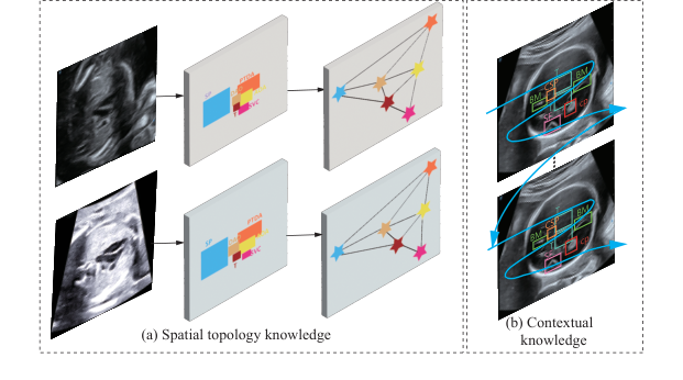 Figure 1. Consistency of two fixed knowledge from human anatomy. (a) Spatial topology knowledge. (b) Contextual knowledge
So, why was this specific mathematical approach the only viable solution? The authors recognized that while recent sequence-modeling architectures like Mamba are fantastic at extracting core semantics from long sequences, standard Mamba has a fatal flaw: it focuses almost entirely on spatial correlations and neglects channel information. In complex medical imaging, this lack of channel mixing causes stability issues in larger networks and severely limits the model's ability to grasp the global picture. To fix this, they designed Circular Channel Mamba (CCM). By extending the selective Structured State Space Model (SSM) mechanism to the channel dimension, CCM captures inter-channel feature dependencies. Mathematically, the hidden state transitions are defined as:
$$h_t = \overline{A}h_{t-1} + \overline{B}x_t$$
This specific formulation allows the model to dynamically filter input information, effectively reducing the sequence modeling compexity from a heavy $O(N^2)$ (typical of standard Transformers) down to a highly efficient $O(N)$.
The comparative superiority of this method lies in its dual-engine structure. Beyond just achieving higher mean average precision (mAP) scores against 9 baseline methods, it is qualitatively superior because it doesn't just "look" at the image; it "reasons" about it. To handle the high-dimensional noise of ultrasounds, the model employs Topological Relationship Reasoning (TRR). It constructs an undirected region-to-region graph $G = \langle \mathcal{N}, \mathcal{E} \rangle$, where nodes represent region proposals and edges represent the relationships between them. By passing spatial coordinates into a Gaussian kernel, the model calculates relationship weights:
$$\omega_m(P(i, j)) = \exp(-\frac{1}{2}(P(i, j) - u_m)^T \Sigma_m^{-1} (P(i, j) - u_m))$$
This means that even if the visual features of a fetal heart are obscured by speckle noise, the Graph Convolutional Network (GCN) can infer its location and class by relyng on the clear presence of surrounding structures. It is a structural advantage that makes it overwhelmingly superior to previous gold standards that treat every bounding box in isolation.
This method perfectly aligns with the harsh constraints of few-shot medical detection. Labeling massive medical datasets requires specialized experts, which can easily cost upwards of USD 150 per hour, making large datasets ethically and financially restrictive. The "marriage" here is between the problem's data scarcity and the solution's use of invariant prior knowledge. Because the model already "knows" the spatial topology of human anatomy via the TRR module, it requires drastically fewer examples to learn how to detect novel classes.
To be honest, I'm not completely sure why the authors didn't explicitly discuss rejecting other popular generative approaches like GANs or Diffusion models for this specific task, as the paper doesn't mention them. However, they do explicitly explain the reasoning behind rejecting previous Mamba-based methods and standard CNNs: those older architecures either fail to mix channel information properly or lack the linear-time selective scanning mechanism required to process complex global contexts efficiently without exploding computational costs. By combining the linear efficiency of CCM with the anatomical constraints of TRR, they created a uniquely robust system tailored specifically for the unforgiving domain of ultrasound imaging.
Mathematical & Logical Mechanism
To understand the brilliance of this paper, we first need to understand the fundamental nightmare of medical ultrasound imaging. Imagine trying to find a specific constellation in a night sky that is constantly shifting, covered in thick clouds, and viewed through a dirty telescope. Ultrasound images are notoriously noisy, blurry, and highly dependent on the doctor holding the probe.
Normally, Deep Learning solves this by looking at hundreds of thousands of labeled examples. But in the medical field, we simply do not have that much annotated data—this is the "few-shot" learning problem. So, how do we teach an AI to find fetal organs with only a handful of examples?
The authors of this paper realized something profound: Human anatomy is a fixed map. Even if the image is terribly blurry, the heart is always in a specific spatial relationship to the spine. By forcing the neural network to obey the invariant laws of human topology and contextual memory, they compensate for the lack of data. To achieve this, they built a dual-core mathematical engine: the Circular Channel Mamba (CCM) for contextual memory, and Topological Relationship Reasoning (TRR) for spatial mapping.
Here is the autopsy of how this system actually works.
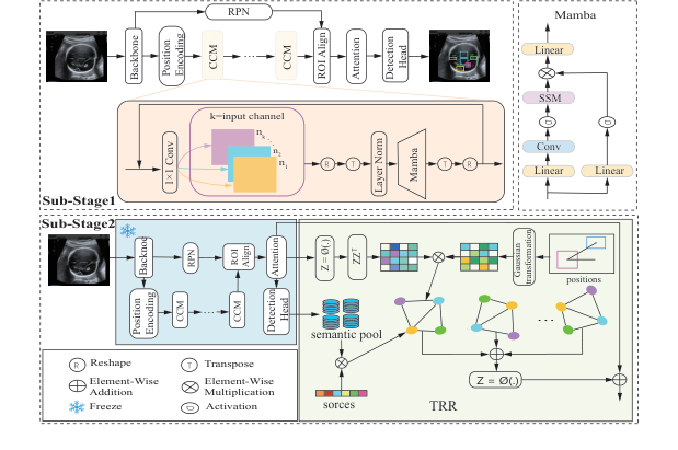 Figure 2. The overall pipeline of the proposed TRR-CCM framework
The Master Equations
The absolute core of this paper is powered by two interconnected mathematical engines.
Engine 1: The Contextual Memory (Structured State Space Model)
This equation allows the model to scan the image and "remember" what it just saw, building a contextual understanding of the tissue.
$$h_t = \overline{A}h_{t-1} + \overline{B}x_t$$
$$y_t = Ch_t$$
Engine 2: The Anatomical Topology (Graph Reasoning)
This is the true breakthrough of the paper. Once the model finds candidate organs, it uses a Gaussian-weighted graph convolution to check if their spatial layout matches human anatomy.
$$f'_m(i) = \sum_{j \in Neighbour(i)} \omega_m(P(i, j)) x_j e_{ij}$$
$$\omega_m(P(i, j)) = \exp\left(-\frac{1}{2}(P(i, j) - u_m)^T \Sigma_m^{-1} (P(i, j) - u_m)\right)$$
Tearing the Equations Apart
Let's dissect every single gear and spring in these equations.
From Engine 1 (The Mamba Context):
* $x_t$: The input at step $t$. Physically, this is a specific patch of the ultrasound image being processed.
* $h_t, h_{t-1}$: The hidden states. This is the model's "working memory." $h_{t-1}$ holds the context of the image patches seen right before the current one.
* $\overline{A}$: The discretized state transition matrix. Think of this as a "forgetting/retention gate." It decides how much of the previous anatomical context should be kept.
* $\overline{B}$: The discretized input matrix. This acts as an "attention filter," deciding how much the current image patch $x_t$ should update the memory.
* $y_t$: The output feature representation for that specific patch, enriched with global context.
* $C$: The output projection matrix that transforms the hidden memory back into a usable visual feature.
* Why addition ($+$) instead of multiplication? The state update uses addition to smoothly accumulate information over time. Multiplication would cause the memory to either explode to infinity or vanish to zero exponentially fast.
From Engine 2 (The Topological Graph):
* $f'_m(i)$: The newly updated, topology-aware feature vector for a candidate organ (node $i$).
* $\sum$: The summation operator. The authors use an integral/summation here rather than a max-pooling or multiplication because they want to accumulate supporting evidence from all surrounding organs. If the heart, lungs, and spine all agree on where they are, their combined voices are added together to boost confidence.
* $Neighbour(i)$: The top-K most relevant candidate organs surrounding node $i$.
* $x_j$: The semantic feature vector of the neighboring organ $j$.
* $e_{ij}$: The edge weight from the sparse adjacency matrix. It represnts the raw, learned relationship strength between organ $i$ and organ $j$.
* $\omega_m(P(i, j))$: The Gaussian kernel weight. This is the "rubber band" of the system. It outputs a high value (close to 1) if the organs are in the correct anatomical position, and a low value (close to 0) if they are not.
* $P(i, j)$: A polar coordinate function returning $(d, \theta)$—the actual measured distance and angle between organ $i$ and organ $j$ in the image.
* $\exp(...)$: The exponential function. It is used to create a smooth, bell-shaped curve. It ensures the spatial weight drops off gracefully rather than abruptly if an organ is slightly shifted due to the ultrasound probe angle.
* $-\frac{1}{2}$: A standard mathematical scaling factor for Gaussian distributions that makes the calculus (gradients) clean and stable during learning.
* $u_m$: A learnable $2 \times 1$ mean vector. Physically, this is the AI's "ideal blueprint." It is the exact distance and angle the AI expects to see between two specific organs based on human anatomy.
* $T$: The transpose operator, necessary to align the vectors for matrix multiplication so the output resolves to a single scalar distance.
* $\Sigma_m^{-1}$: The inverse of a learnable $2 \times 2$ covariance matrix. Physically, this is the "wiggle room" or tolerance. Some organs shift around a lot depending on the fetus's position (high variance), while others are rigidly fixed (low variance). This matrix scales the penalty accordingly.
Step-by-Step Flow: The Assembly Line
Let’s trace a single abstract data point—a blurry blob that might be a fetal heart—through this architecure.
- Raw Extraction: The ultrasound image enters the backbone network. Our blurry blob is converted into a raw mathematical tensor (a grid of numbers).
- Contextual Sweeping (CCM): The tensor is sliced into sequences and fed into the Circular Channel Mamba. The $\overline{A}$ and $\overline{B}$ matrices sweep across the image. As the math engine processes the blob, it adds context: "I just passed a spine-like texture, so this blob is likely in the chest cavity." The blob becomes $y_t$.
- Graph Construction (TRR): The blob is now a "region proposal" (node $i$). The system looks at nearby blobs (node $j$). It calculates $P(i, j)$, finding that node $j$ is 5 centimeters away at a 45-degree angle.
- Anatomical Interrogation: This $(d, \theta)$ coordinate is fed into the Gaussian kernel $\omega_m$. The kernel compares it against the blueprint $u_m$. Because a heart and a spine should be at a 45-degree angle in this specific view, the term $(P(i, j) - u_m)$ becomes nearly zero.
- Evidence Aggregation: Because the distance is near zero, the $\exp(0)$ evaluates to 1. The semantic data $x_j$ of the spine is multiplied by 1 and added ($\sum$) to our blob $i$.
- Final Output: Our blurry blob is no longer just a blob. It is now mathematically fused with the absolute certainty of its surrounding anatomical neighbors. The model confidently detects it as the fetal heart.
Optimization Dynamics
How does this mechanical beast actually learn from just a few images?
In standard few-shot learning, the loss landscape is chaotic. Because there is so little data, the model easily overfits, finding fake patterns (like memorizing the static noise of a specific ultrasound machine). The gradients usually bounce around wildly.
However, the TRR module acts as a massive gravitational anchor on the loss landscape. During training, the model uses a standard SGD (Stochastic Gradient Descent) optimizer. The magic happens in the gradients flowing back into $u_m$ and $\Sigma_m$.
Initially, $u_m$ (the expected organ locations) is randomized. The model might guess that the heart is outside the body, resulting in a massive classification error. The loss function sends a steep gradient back, forcefully updating $u_m$ to reflect the true spatial coordinates found in the few labeled examples.
Because human anatomy is highly consistent, $u_m$ converges very quickly. Once $u_m$ is locked in, the $\Sigma_m$ (covariance) matrix learns the natural elasticity of the fetal tissue. This fundamentally reshapes the optimization dynamcis: instead of forcing the neural network to learn what a heart looks like from scratch using millions of pixels, the gradients are channeled into learning where the heart should be relative to other structures. This topological constraint smooths out the local minima, allowing the model to generalize beautifully across different ultrasound machines and patients, even when it has only seen 3 or 5 examples.
Results, Limitations & Conclusion
Imagine trying to find a specific, tiny structure in a grainy, black-and-white TV static image. Now imagine that someone’s life depends on you finding it accurately. This is the daily reality of ultrasound image analysis.
To understand the brilliance of this paper, we first need to establish some ground truths about modern artificial intelligence. Deep learning models are incredibly smart, but they are also notoriously data-hungry. To teach an AI to find a fetal heart defect, you typically need thousands of images, painstakingly annotated by medical experts. This isn't just tedious; it's incredibly expensive, sometimes costing upwards of \$150 per hour for a specialized radiologist's time. Furthermore, strict privacy regulations often make gathering massive medical datasets impossible.
This brings us to the constraint: Few-Shot Learning (FSL). FSL is the AI equivalent of showing a brilliant student just three or five examples of a problem and expecting them to ace the final exam. While FSL has seen success in general image classification, applying it to object detection (finding bounding boxes around multiple objects) in ultrasound images is a nightmare. Ultrasounds suffer from severe domain shifts—different machines, different probe angles, and inherent speckle noise.
So, what was the authors' "Aha!" motivation? They realized that while ultrasound images are messy and unpredictable, human anatomy is not. The spatial topology (where organs are located relative to one another) and the anatomical context are invariant. The authors hypothesized that if they could mathematically hardcode this invariant human anatomy into the neural network, the model wouldn't get confused by the noise.
The Mathematical Interpretation: TRR-CCM
To solve this, the authors engineered a dual-engine architecure called TRR-CCM (Topological Relationship Reasoning with Circular Channel Mamba). Let's break down exactly how they translated biology into mathematics.
1. Circular Channel Mamba (CCM)
Standard vision models often struggle to see the "big picture" without requiring massive computational power. The authors turned to a cutting-edge sequence modeling framework called Mamba, which is based on Structured State Space Models (SSMs). A standard SSM maps a 1D sequence $x(t)$ to $y(t)$ through a hidden state $h(t)$:
$$h_t = \overline{A}h_{t-1} + \overline{B}x_t, \quad y_t = C h_t$$
where $\overline{A}$ and $\overline{B}$ are discrete-time parameters.
However, standard Mamba has a fatal flaw for vision: it ignores channel information (the depth of the feature maps). To fix this, the authors invented CCM. Before feeding the image into Mamba, they force the network to aggregate cross-channel information using a convolution operation:
$$\overline{X}(c, m, n) = \sum_{i=0}^{K-1} \sum_{j=0}^{K-1} X_{c, m+i, n+j} \cdot W_{c, i, j}$$
This equation essentially says: "Before looking at the sequence, blend the features across all channels so no context is lost." They then encode this global context through the Mamba block:
$$\hat{X} = Mamba(LN(X^T))$$
Finally, they add this enriched feature back to the original input via a residual connection: $X_{out} = CCM(X + \hat{X}')$.
2. Topological Relationship Reasoning (TRR)
This is where the anatomical map is built. The authors use a Graph Convolutional Network (GCN) where each "node" is a potential anatomical structure. But how does the AI know how these structures relate to each other?
They use polar coordinates to calculate the exact distance $d$ and angle $\theta$ between any two region proposals $(x_i, y_i)$ and $(x_j, y_j)$:
$$d = \sqrt{(x_i - x_j)^2 + (y_i - y_j)^2}, \quad \theta = \arctan\left(\frac{y_j - y_i}{x_j - x_i}\right)$$
They don't just feed these raw numbers into the network. They pass this topological data through a Gaussian kernel to generate relationship weights:
$$\omega_m(P(i, j)) = \exp\left(-\frac{1}{2}(P(i, j) - u_m)^T \Sigma_m^{-1} (P(i, j) - u_m)\right)$$
This beautiful equation acts as a dynamic relevance filter. It mathematically dictates how much attention one organ should pay to another based on their expected anatomical distance and angle. Finally, the information is aggregated across the graph:
$$f'_m(i) = \sum_{j \in Neighbour(i)} \omega_m(P(i, j)) x_j e_{ij}$$
The Experimental Arena and The "Victims"
The authors didn't just claim their math worked; they architected a ruthless experimental gauntlet to prove it. They tested their model on two distinct, highly complex datasets: TT (fetal brain) and 3VT (fetal heart). They evaluated the model under extreme starvation conditions: 1, 2, 3, 5, and 10-shot settings.
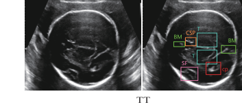 Figure 3. Examples of two datasets
The "victims" were 9 state-of-the-art Few-Shot Object Detection baselines, including heavyweights like TFA, FSCE, DeFRCN, and TKR.
The definitive, undeniable evidence of their success wasn't just the overall leaderboard—it was the ablation study (Table 3). By stripping the model down to its base components, they proved that adding just CCM or just TRR improved perfromance, but combining them created a synergistic explosion. For instance, in the 1-shot TT dataset, the baseline scored 67.4%. Adding CCM bumped it to 68.8%, adding TRR bumped it to 68.5%, but combining them rocketed the score to 71.3%.
To be honest, I'm not completely sure why the TRR module outperformed the CCM module so heavily on the heart dataset (3VT) compared to the brain dataset (TT), but if I had to deduce, it likely stems from the fact that the fetal heart's three-vessel trachea view has a much more rigid, predictable spatial geometry than the brain structures, making the polar-coordinate graph reasoning exceptionally lethal there.
Discussion Topics for Future Evolution
Based on the brilliant foundations laid in this paper, here are several avenues for future critical thinking and evolution:
- The Paradox of Pathological Anomalies: The core strength of TRR is its reliance on invariant human anatomy. But what happens when the anatomy is fundamentally wrong? If a fetus has a severe congenital defect (e.g., transposed vessels), will the TRR's rigid Gaussian kernel suppress the detection because the realtionships violate the "normal" topological prior? We must discuss how to make the graph reasoning flexible enough to detect anomalies without losing its noise-filtering robustness.
- Cross-Modality Topological Projection: Could we extract the pristine, perfect topological graphs from high-resolution MRI or CT scans and mathematically project them into the latent space of this ultrasound model? If the spatial math is truly invariant, we shouldn't need to learn the graph from noisy ultrasounds at all; we could import the "ground truth" graph from a superior imaging modality.
- The Limits of 1D Sequence Models in 2D Space: Mamba is inherently a 1D sequence model. The authors flattened the 2D ultrasound features to feed them into CCM. While computationally efficient, flattening destroys native 2D spatial contiguity. A fascinating future direction would be formulating a native 2D continuous state-space model that doesn't require sequence flattening, potentially capturing anatomical boundaries with even greater precision.
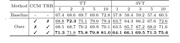 Table 3. shows the ablation studies of the CCM and TRR modules on data split 1 of the TT and 3VT datasets. As shown in Table 3, TRR outperformed CCM on the 3VT dataset, while CCM outperformed TRR on the TT dataset. Both components improve our model’s performance, validating the effectiveness of TRR-CCM. Specifically, the addition of CCM only achieves a significant im- provement over the baseline method by 1.4% to 9.4% on TT dataset, and 5.9% to 12.1% on 3VT dataset, respectively. Only by adding the TRR, it outperforms the baseline on most of the shots of TT, while the 3VT dataset sees an improve- ment of over 5.7% in all cases. When both CCM and TRR are included, our method boosts by 3.9%, 3.2%, 6.1%, 10.2%, and 8.2% in the cases of 1, 2, 3, 5, and 10 shot on data split 1 of TT, respectively
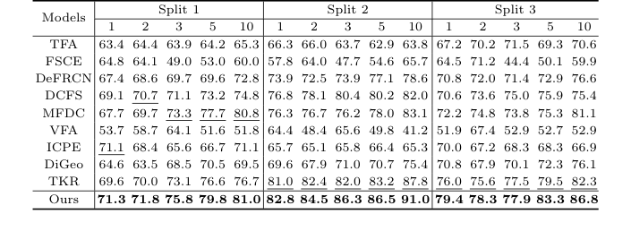 Table 1. Detection results for the TT dataset under the three settings. Bold and underlined numbers denote the 1st and 2nd scores
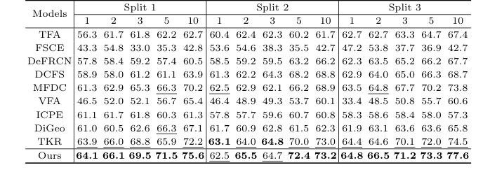 Table 2. Detection results for the 3VT dataset under the three settings. Bold and underlined numbers denote the 1st and 2nd scores