One-shot active learning for vessel segmentation
New AI learns from tiny, smart samples, saving time & resources for better disease insights.
Background & Academic Lineage
In the field of medical imaging, mapping out the brain's blood vessels—a process known as vessel segmentation—is a critical step for understanding cerebral functions and diagnosing severe neurological disorders like strokes. Historically, as deep learning models became the gold standard for this task, a massive bottleneck emerged: these models are incredibly data-hungry. They require thousands of 3D brain scans to be meticulously annotated by medical experts. Manually tracing intricate, microscopic vascular networks is not only exhausting but also prohibitively expensive, sometimes costing the equivalent of \$150 or more in expert labor per single scan.
To alleviate this, the field turned to Active Learning (AL), a paradigm where the AI identifies the most informative unlabeled samples and asks the human expert to label only those. However, classical AL is highly iterative. It requires a cycle of training the model, pausing to ask the expert for a label, retraining the model, and asking again. This constant back-and-forth demands the continuous availability of clinical experts and incurs massive computational overhead, making real-time clinical application nearly impossible.
The fundamental limitation that forced the authors to write this paper lies in the flaws of the next evolutionary step: One-Shot Active Learning (OSAL). While OSAL attempts to select a minimal set of samples in a single pass (eliminating the back-and-forth), previous OSAL models were essentially "black boxes." They relied on generic data augmentation or contrastive learning without any explicit mechanism to understand the actual anatomy of the brain. Specifically, they completely ignored the recurring, tree-like structurs of blood vessels. Because these older models couldn't interpret why they were selecting certain data points, they often picked non-represntative samples. This led to models that failed to generalize to new, unseen patient data. The authors realized that to fix this, they needed an OSAL framework tailored specifically to the unique, recurring geometry of brain vessels.
To help you intuitively understand how the authors solved this, here are the core concepts translated from highly specialized domain terms into everyday analogies:
- One-Shot Active Learning (OSAL): Imagine you are grocery shopping for a massive, complex feast, but you are only allowed to visit the store exactly once. Instead of running back to the store every time you realize you need a missing ingredient (which is how iterative Active Learning works), you carefully analyze your recipe beforehand and buy a perfectly diverse, minimal set of ingredients in a single, highly efficient trip.
- Dictionary Learning & Atoms: Think of this like a master builder's Lego set. Instead of trying to memorize the exact shape of every single toy castle or spaceship ever built, the AI just learns a small set of fundamental Lego bricks (called "atoms"). By combining these basic bricks in different ways, the AI can reconstruct any complex blood vessel shape it encounters.
- Latent Space: Imagine a massive, magical library where books aren't sorted alphabetically, but by how similar their plots are. A latent space is a mathematical "room" where the AI places image patches. Patches with similar vessel patterns are placed right next to each other, while completely different patterns are pushed far away, making it easy to see the big picture of the data.
- Siamese Encoder: Picture twin detectives working on the same case. They are handed two different clues (image patches). If the clues belong to the same suspect (the same vessel pattern), the detectives tie them together with a short string. If they belong to different suspects, they push them apart. This algoritm ensures the latent space is perfectly organized and highly discriminative.
Here is a breakdown of the key mathematical notations used to formulate and solve this problem:
| Notation | Description |
|---|---|
| $\mathcal{I}$ | The labeled dataset containing images and their corresponding expert annotations. |
| $\mathbf{I}$ | A specific 3D volumetric image (e.g., an MRI brain scan) from the dataset. |
| $\mathbf{L}$ | The ground-truth label map associated with image $\mathbf{I}$. |
| $H \times W \times S$ | The dimensions of the image (Height, Width, and number of Slices). |
| $X_k, Y_k$ | Non-overlapping 2D image patches and their corresponding label patches. |
| $\mathcal{Y}_{\mathcal{I}}$ | The set of binary vessel annotated patches extracted from the dataset. |
| $\mathbf{B}$ | An over-complete dictionary containing the fundamental building blocks (atoms) of tree-like branching patterns. |
| $\mathbf{z}$ | A sparse vector containing the representation coefficients (determining which atoms are activated). |
| $\hat{\mathbf{B}}, \hat{\mathbf{Z}}$ | The learned dictionary and the learned sparse latent vectors obtained after optimization. |
| $\lambda$ | A regularization parameter that controls the sparsity of the representation vectors (forcing the model to use as few atoms as possible). |
| $c_i$ | The k-means cluster label assigned to a specific annotation and its corresponding image patch. |
| $\mathcal{E}_1, \mathcal{R}_1$ | The linear encoder and decoder used to map patches to sparse latent vectors and reconstruct them. |
| $\mathcal{E}_s$ | The Siamese encoder network used to generate the final informative latent space for MRI patches. |
| $\mathcal{I}^U$ | A new dataset of unlabeled images that the model needs to sample from. |
| $n$ | The minimal subset of brain patches selected by the framework to be sent to the human expert for annotation. |
| $\Phi$ | The final brain vessel segmentation model trained using the newly annotated patches. |
By combining these elements, the authors successfully created V-DiSNet, a system that mathematically models the recurring patterns of blood vessels as $$ \mathbf{Y} = \mathbf{B}\mathbf{z} $$ and uses this understanding to pick the absolute best $n$ patches for a human to label, achieving near full-dataset performance with only 30% of the data labeled.
Problem Definition & Constraints
To understand the exact problem this paper tackles, we first need to look at the starting line and the finish line.
The Input (Current State): We start with a massive, unlabeled dataset of 3D brain scans—specifically Magnetic Resonance Angiography (MRA) images. Mathematically, this is a set of unlabeled volumetric images $I^U = \{I_j\}_{j=1}^M \subset \mathbb{R}^{H \times W \times S}$.
The Output (Goal State): The goal is a fully trained, highly accurate deep learning model capable of segmenting (precisely outlining) the intricate, tree-like blood vessels in the brain. However, there is a catch: we want to achieve this by having human medical experts manually annotate only a tiny, carefully selected fraction of the original data (e.g., just 30% or even less).
The Missing Link: The mathematical gap between the input and the goal is the selection mechanism. How do you mathematically guarantee that the small handful of images you ask the doctors to label are the most informative ones, before you actually know what is inside them? The authors hypothesize that brain vessels are built from recurring, hierarchical branching patterns. Therefore, any vascular tree image $\mathbf{Y}$ can be modeled as a linear combination of fundamental building blocks (a dictionary $\mathbf{B}$) and sparse coefficients ($\mathbf{z}$), such that $\mathbf{Y} = \mathbf{B}\mathbf{z}$. The missing link this paper bridges is figuring out how to learn this hidden dictionary of vessel patterns and map unlabeled images into a latent space where we can mathematically sample the most diverse, represntative patches in a single pass.
This brings us to the painful dilemma that has trapped previous researchers.
In the world of machine learning, reducing the need for human labels usually relies on Active Learning (AL). Traditional AL is an iterative process: the model trains on a few images, figures out what it is most confused about, asks a human oracle to label those specific confusing images, and then retrains.
* The Trade-off: You get high accuracy with few labels, but you incur massive computional costs from constantly retraining the model. Worse, it requires a medical expert to be continuously on standby to answer the algorithm's queries, which is practically impossible in real clinical settings.
To fix this, researchers invented One-Shot Active Learning (OSAL), which attempts to select the entire batch of informative samples in one single go, eliminating the iterative retraining loop.
* The New Dilemma: Existing OSAL methods rely on generic, "black-box" math (like contrastive learning or variational autoencoders) that are completely blind to the actual physical anotomy of the brain. They do not understand that blood vessels are continuous, recurring tubular structures. If you use these generic methods to pick samples in one shot, you risk selecting a batch of images that completely misses crucial anatomical variations. You trade computational efficiency for a model that fails to generalize to unseen data because its training set wasn't truly representative of the complex vascular tree.
To solve this, the authors hit several harsh, realistic walls:
- The Hidden Dictionary Constraint: The fundamental building blocks (the "atoms") of brain vessels are not directly observed. To find them, the authors had to solve a highly constrained optimization problem to minimize the reconstruction error while forcing the representation to be sparse. They had to mathematically define this as:
$$ \hat{\mathbf{B}}, \hat{\mathbf{Z}} = \min_{\mathbf{B}, \mathbf{Z}} \|\mathcal{Y}_{\mathcal{I}} - \mathbf{B}\mathbf{Z}\|_2^2 $$
subject to the strict sparsity constraint $\|\mathbf{Z}\|_1 < \lambda$. Solving this requires specialized, complex algorithms like the learned Iterative Shrinkage Thresholding Algorithm (LISTA). - Extreme Data Sparsity and Complexity: Blood vessels are incredibly thin, intricate, and sparse compared to the surrounding brain tissue. Capturing their connectivity and tubular shape means standard pixel-by-pixel analysis isn't enough; the model must somehow understand the geometry of a branching tree.
- Hardware and Dimensionality Limits: 3D volumetric brain scans are massive. Processing full 3D patches to learn these sparse dictionaries is incredibly memory-intensive. To be honest, I'm not completely sure if it was strictly a GPU memory limit or a mathematical complexity limit, but the authors explicitly acknowledge a harsh compromise: they had to slice the 3D volumes into 2D patches to make the dictionary learning tractable. This reliance on 2D patches means they risk losing some of the global 3D spatial connectivity of the vascular tree—a physical constraint they had to accept to make the math work within reasonable computational bounds.
Why This Approach
The authors of this paper reached a critical "aha!" moment when they realized that existing state-of-the-art (SOTA) One-Shot Active Learning (OSAL) frameworks were fundamentally blind to human anatomy. Traditional methods rely heavily on generic self-supervised learning, Variational Autoencoders (VAEs), or contrastive learning. While these approaches are excellent at finding statistical outliers in standard image datasets, they treat brain scans as generic pixel distributions. They completely fail to account for the recurring, tree-like, tubular structures of brain vessels.
Because of this anatomical blindness, standard deep learning models could not guarantee that the selected samples were actually meaningful or represntative of the full vascular tree. The authors recognized that to solve this, they needed a mathematical model that inherently understood hierarchical branching. This is why Dictionary Learning combined with sparse coding was the only viable solution. Based on the theoretical foundation that a vascular tree can be modeled as a linear combination of fundemental building blocks, they formulated the problem to extract these hidden "atoms" of vessel patterns.
Mathematically, they defined this extraction by solving the following optimization problem:
$$ \hat{\mathbf{B}}, \hat{\mathbf{Z}} = \min_{\mathbf{B},\mathbf{Z}} \|\mathcal{Y}_{\mathcal{I}} - \mathbf{B}\mathbf{Z}\|_2^2 $$
subject to the sparsity constraint $\|\mathbf{Z}\|_1 < \lambda$. Here, $\mathcal{Y}_{\mathcal{I}}$ represents the observed vessel patches, $\mathbf{B}$ is the over-complete dictionary of vessel patterns, and $\mathbf{Z}$ contains the sparse representation coefficients. By using the learned Iterative Shrinkage Thresholding Algorithm (LISTA), they could efficiently solve this, forcing the network to learn a highly compressed, sparse latent vector where each active element corresponds to a specific physical trait of a blood vessel (like its shape, size, or connectivity).
When benchmarking this approach against previous gold standards, the comparative superiority of V-DiSNet goes far beyond simple performance metrics like Dice scores. The true structural advantage lies in its interpretability and efficiency. Standard OSAL methods are black boxes; they cannot explain why one data point is prioritized over another. In contrast, V-DiSNet's sparse latent space is entirely transparent. If you deactivate a specific "atom" in the latent vector, a specific part of the vessel physically alters or disappears in the reconstruction. Furthermore, by mapping high-dimensional volumetric brain patches into this sparse latent space and applying k-means clustering, the model drastically reduces the search space compexity. Instead of blindly evaluating the distance between millions of high-dimensional patches, the system groups them by structural similarity and uses a stratified Farthest Point Sampling (FPS) algorithm to pick exactly what it needs, effectively bypassing the massive computational overhead of traditional sampling.
This chosen method perfectly aligns with the harsh constraints of the medical field. In a clinical setting, doctors and expert annotators have severely limited time. Iterative Active Learning—which requires a human to label a few images, wait for the model to retrain, and then label more—is practically useless due to its continuous overhead. The problem demanded a "one-shot" solution (a single labeling round) that still captured the vast diversity of brain vessels. The "marriage" here is beautiful: the harsh constraint of zero iterative feedback is overcome by the dictionary learning's unique ability to guarantee that the minimal subset of patches sent to the oracle covers every possible structural variation of the vascular tree.
If the authors had attempted to use other popular generative approaches, such as GANs or standard Diffusion models, they would have failed. While a GAN might generate highly realistic synthetic blood vessels, it does not provide an explicit, interpretable mechanism to measure the structural diversity of an unlabeled dataset. GANs and Diffusion models map data to continuous, often entangled latent spaces where isolating a specific "branching pattern" is incredibly difficult. By rejecting these black-box generative models in favor of sparse Dictionary Learning, the authors ensured that their sampling strategy was driven by actual, verifiable vascular anatomy rather than opaque statistical variance.
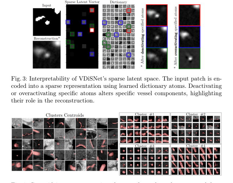 Figure 4. Centroid images representing clusters of vessel patches extracted from 3D MRA brain image volumes (left); and examples of clusters of brain patches characterized by similar vessel features, such as shape, size, or position (right)
Mathematical & Logical Mechanism
At the heart of this paper lies a mathematical engine designed to distill the chaotic, branching complexity of brain blood vessels into a clean, manageable vocabulary of fundamental shapes. To achieve this, the authors rely on a classic formulation from sparse dictionary learning, adapted here as a pretext task to build an interpretable latent space.
Here is the master equation that powers the framework:
$$ \hat{\mathcal{B}}, \hat{\mathbf{Z}} = \min_{\mathcal{B}, \mathbf{Z}} \|\mathcal{Y}_{\mathcal{I}} - \mathcal{B}\mathbf{Z}\|_2^2 $$
subject to the constraint:
$$ \|\mathbf{Z}\|_1 < \lambda $$
Let's tear this equation apart piece by piece to understand exactly what it is doing:
- $\hat{\mathcal{B}}, \hat{\mathbf{Z}}$: These are the final, optimized outputs of the engine. $\hat{\mathcal{B}}$ is the learned "dictionary"—think of it as a catalog of fundamental, recurring vessel building blocks (like a straight tube, a sharp curve, or a Y-shaped bifurcation). $\hat{\mathbf{Z}}$ is the sparse coefficient matrix, which acts as the specific recipe telling the system which blocks to use for each image.
- $\min_{\mathcal{B}, \mathbf{Z}}$: This is the optimization directive. It tells the mathematical engine to continuously tweak both the dictionary $\mathcal{B}$ and the recipes $\mathbf{Z}$ until the expression to its right reaches the lowest possible value.
- $\mathcal{Y}_{\mathcal{I}}$: The input data matrix. Physically, these are the actual, observed binary image patches of brain vessels extracted from the dataset.
- $-$ (Subtraction): Used here to calculate the residual. It measures the exact gap between the real vessel patch and the model's artificial attempt to recreate it.
- $\mathcal{B}\mathbf{Z}$: The reconstructed data. The authors use matrix multiplication here because it perfectly models a linear combination. The matrix multiplication scales each dictionary atom in $\mathcal{B}$ by the intensity weight specified in $\mathbf{Z}$, and then adds them all together. Addition is used to overlay these fundamental shapes on top of one another to build the final complex vessel structure.
- $\| \cdot \|_2^2$: The squared L2 norm. Mathematically, it sums the squared differences of all pixels between the real and fake patches. Physically, it acts as a rubber band pulling the model toward high fidelity. The authors used a squared L2 norm instead of an absolute L1 norm here because squaring heavily penalizes large, glaring errors (like missing a thick vessel entirely), forcing the model to capture the overall macro-structure accurately.
- $\|\mathbf{Z}\|_1 < \lambda$: The sparsity constraint using the L1 norm. Mathematically, it sums the absolute values of the coefficients in the recipe. Physically, it acts as a strict budget. It forces the model to use the absolute minimum number of dictionary atoms to reconstruct the image.
- $\lambda$: The regularization parameter. It is the tuning knob that dictates how strict the sparsity budget is. A higher $\lambda$ forces a sparser represntation, meaning the model can only pick a tiny handful of atoms per patch.
Step-by-step Flow
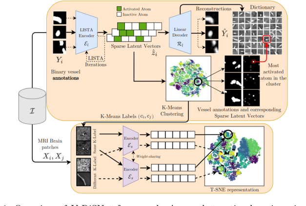 Figure 1. Overview of V-DiSNet framework: A one-shot active learning pipeline that leverages dictionary learning to capture intrinsic vessel patterns, constructs an informative latent space via a Siamese encoder, and applies diversity-based sampling to select a minimal yet representative set of vessel patches for efficient brain vessel segmentation
Imagine an automated assembly line designed to build complex vascular trees out of simple Lego bricks.
First, a raw, unlabeled image patch of a brain vessel $Y_i$ enters the factory. It gets fed into a linear encoder (acting as a scanner). This scanner looks at the complex vessel and generates a sparse blueprint vector $\hat{z}_i$. Because of the strict L1 budget we discussed, this blueprint is mostly zeros—it is forced to be highly selective, activating only a few essential components.
Next, this blueprint is sent to the dictionary $\mathcal{B}$, which is the warehouse storing the fundamental vessel parts. The non-zero values in $\hat{z}_i$ act as mechanical levers. If the blueprint has a value of $0.8$ at position 5, it pulls "Atom 5" (perhaps a specific Y-branch shape) from the warehouse and scales its intensity by $0.8$.
Finally, these selected, scaled parts are stacked on top of each other to build the final recontructed patch $\hat{Y}_i$. The system then looks at the difference between the original patch and this new construction, calculates the error, and sends a signal back to the start of the line to adjust the scanner and the warehouse inventory for the next round.
Optimization Dynamics
How does this mechanism actually learn and converge? The optimization landscape here is a classic tug-of-war. The L2 norm wants to perfectly recreate the image, which usually means using every tool available (resulting in a dense $\mathbf{Z}$). But the L1 constraint is a strict manager demanding efficiency, forcing most of $\mathbf{Z}$ to zero.
To solve this non-trivial optimization problem, the authors don't just use standard gradient descent. They use LISTA (Learned Iterative Shrinkage Thresholding Algorithm). LISTA takes a traditional mathematical solver and unrolls its iterative steps into the layers of a neural network.
During training, the loss landscape is shaped like a smooth, multidimensional bowl (from the L2 norm) intersecting with a sharp, multi-dimensional diamond (from the L1 norm). As the gradients flow backward through the unrolled LISTA network, the "shrinkage" operation acts like a pair of scissors. It looks at the gradient updates and literally clips the small, insignificant weights to exactly zero.
Over time, this dynamic forces the dictionary $\mathcal{B}$ to discard useless noise and only keep the most universally applicable vessel shapes. Simultaneously, the encoder learns to navigate this diamond-shaped loss landscape to pick the most efficent combinations instantly. Once this latent space is fully formed and clustered, the active learning framework can easily sample from different clusters, guaranteeing that the human annotator receives a perfectly diverse set of vessel geometries to label.
Results, Limitations & Conclusion
Imagine you are tasked with mapping the intricate plumbing system of a massive, complex city. You cannot see the pipes directly; you only have blurry radar scans. To build an accurate map, you need an expert plumber to look at the scans and trace every single pipe by hand. This is incredibly expensive—costing perhaps \$500 per scan in expert medical time—and painfully slow.
In the realm of medical imaging, this "plumbing system" is the human brain's vascular network, and the "radar scans" are Magnetic Resonance Angiography (MRA) images. Deep learning models are fantastic at mapping these vessels, but they are notoriously data-hungry. They require fully labeled datasets to learn, meaning human doctors must spend countless hours annotating 3D brain scans voxel by voxel.
To bypass this bottleneck, scientists use Active Learning (AL). Instead of labeling everything, the AI looks at the data and asks the human to label only the most confusing or informative parts. However, traditional AL is iterative: the AI asks for a few labels, trains itself, realizes it needs more, and asks again. This constant back-and-forth is highly impractical in busy clinical settings. Enter One-Shot Active Learning (OSAL), where the AI selects a single, minimal batch of data to be labeled all at once.
The constraint the authors of this paper had to overcome is that existing OSAL methods are essentially blind to anatomy. They pick data points based on statistical anomalies or pixel variances, completely ignoring the fundemental reality that blood vessels are continuous, tree-like, tubular structures. If an OSAL model just picks random "hard" patches, it might miss the recurring branching patterns that define the vascular system, leading to an AI that fails to generalize.
The Mathematical Core: Decoding the Anatomy
To solve this, the authors created V-DiSNet (Vessel-Dictionary Selection Net). Their brilliant insight was to treat the complex vascular tree not as a random assortment of pixels, but as a language built from a finite alphabet of basic shapes—like straight tubes, Y-junctions, and curves.
Mathematically, they modeled a vascular image patch $\mathcal{Y}$ as a linear combination of these basic building blocks. They defined an over-complete "dictionary" $\mathcal{B}$ (the alphabet of shapes) and a sparse vector $\mathbf{Z}$ (the specific recipe of which shapes to use and how strongly to weight them).
Because they didn't know the dictionary beforehand, they had to learn it from an existing labeled dataset. They framed this as an optimization problem:
$$ \hat{\mathcal{B}}, \hat{\mathbf{Z}} = \min_{\mathcal{B}, \mathbf{Z}} \|\mathcal{Y}_{\mathcal{I}} - \mathcal{B}\mathbf{Z}\|_2^2 $$
subject to the constraint:
$$ \|\mathbf{Z}\|_1 < \lambda $$
Here is what this elegantly means: The algorithm tries to find the optimal dictionary ($\hat{\mathcal{B}}$) and the optimal recipe ($\hat{\mathbf{Z}}$) so that when you multiply them together, the difference between the reconstructed image and the real annotated image ($\mathcal{Y}_{\mathcal{I}}$) is as close to zero as possible (minimized by the squared L2 norm).
The crucial part is the constraint $\|\mathbf{Z}\|_1 < \lambda$. This is a sparsity constraint. It forces the model to use the absolute minimum number of "ingredients" from the dictionary to reconstruct the vessel. By forcing sparsity, the model cannot just memorize the image; it is forced to discover the true, underlying, recurring anatomical patterns (the "atoms").
Once these atoms are learned, the authors use a Siamese neural network architecure to map new, unlabeled MRI patches into a latent space (a mathematical representation space). Patches with similar vessel structures are pulled close together, while patches with different structures are pushed apart. Finally, they use a Farthest Point Sampling (FPS) algorithm to select a tiny, highly diverse set of patches spread evenly across this space. This guarantees that the human expert is asked to label a perfectly represntative cross-section of every type of vessel geometry present in the brain.
The Experimental Architecture: Ruthless Proof of Concept
The authors did not just throw their model at a dataset and report a minor accuracy bump. They architected a rigorous stress test to prove their sampling mechanism was vastly superior to existing paradigms.
Their "victims" were standard Random Sampling (R-W) and three state-of-the-art OSAL baselines: RA (Representative Annotation), CA (Contrastive Active Learning), and AET (Active Learning via Epistemic and Aleatoric Uncertainty). They deployed these models across three distinct, publicly available 3D MRA datasets (OASIS-3, SMILE-UHURA, and CAS) to ensure the results weren't a fluke of one specific scanner type.
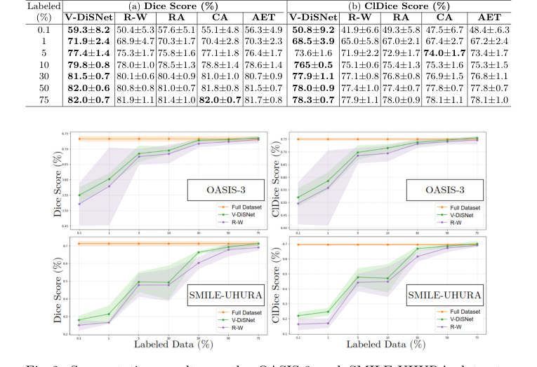 Figure 2. Segmentation results on the OASIS-3 and SMILE-UHURA datasets, showing Dice scores (left) and ClDice scores (right) for different percentages of sample and annotated patches
The definitive evidence of V-DiSNet's superiority was found in the ultra-low data regimes. The authors starved the models, giving them access to only 0.1%, 1%, 5%, and 10% of the labeled data. In these extreme conditions, V-DiSNet systematically crushed the baselines.
Furthermore, they didn't just measure standard pixel overlap (Dice score). They utilized the clDice metric, which specifically measures the topological correctness and connectivity of tubular structures. This proved that V-DiSNet wasn't just guessing pixels better; it was actually preserving the continuous, pipe-like integrity of the blood vessels. The ultimate mic-drop moment in their data is that with a mere 30% of the dataset labeled, V-DiSNet achieved nearly the exact same segmentation performance as a model trained on 100% of the fully annotated data.
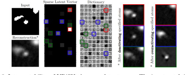 Figure 3. Interpretability of VDiSNet’s sparse latent space. The input patch is en- coded into a sparse representation using learned dictionary atoms. Deactivating or overactivating specific atoms alters specific vessel components, highlighting their role in the reconstruction
To prove their mathematical latent space wasn't just a black box, they performed an interpretability experiment. By manually deactivating specific "atoms" in their learned dictionary $\mathbf{Z}$, they showed that specific physical features of the reconstructed blood vessels (like a specific branch or curve) would disappear. This undeniably proved that their math had successfully isolated the physical geometry of human vasculature.
Discussion Topics for Future Evolution
Based on the profound implications of this paper, here are several avenues for future exploration and critical thought:
-
From 2D Patches to 3D Global Topology:
The current framework operates on 2D patches extracted from 3D volumes. While effective locally, this risks losing the global continuity of the vascular tree (e.g., a long artery spanning multiple patches). How can we evolve the dictionary learning equation to natively process 3D volumetric graphs without causing computational costs to explode? Could we integrate topological data analysis (TDA) to enforce global connectivity constraints during the sampling phase? -
Cross-Modality Anatomical Transferability:
V-DiSNet learns its dictionary from MRA scans. However, the fundamental shape of blood vessels remains the same whether viewed through MRA, CT Angiography (CTA), or ultrasound. Could a universal "Vessel Dictionary" be trained once and then transferred across entirely different imaging modalities? This would allow a hospital to use a dictionary learned from cheap, abundant MRA data to perform One-Shot Active Learning on rare, expensive, or novel imaging types. -
Integrating Physics and Hemodynamics:
Currently, the dictionary atoms are learned purely from static spatial geometry. But blood vessels are shaped by the fluid dynamics of the blood flowing through them. If we were to inject physics-informed neural networks (PINNs) into the latent space generation, could we force the Siamese network to cluster vessels not just by shape, but by their hemodynamic properties (e.g., shear stress or flow velocity)? This could revolutionize how we sample data for predicting aneurysms or strokes.
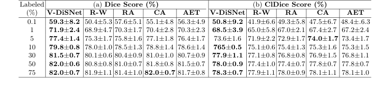 Table 1. Segmentation performance on 15 CAS dataset test patients at various labeling percentages. Eight experiments with distinct random seeds were run for each fraction and model. Results were averaged and standard deviations computed across test patients