Single Image Test-Time Adaptation via Multi-View Co-Training

Background & Academic Lineage

Medical imaging AI has long struggled with a frustrating reality: a deep learning model trained to detect tumors at Hospital A will frequently fail when deployed at Hospital B. This happens because different hospitals use different MRI scanners (e.g., GE vs. Siemens), varying magnetic field strengths, and distinct software protocols. In the academic field of computer vision and medical image analysis, this discrepancy is known as "domain shift."

Historically, researchers tried to solve this by collecting massive datasets from the new hospital to retrain or fine-tune the model. However, in a real-world clinical enviornment, doctors need immediate, on-the-fly analysis for a single patient who just walked into the clinic. You cannot tell a patient to wait weeks while the hospital collects a thousand more scans to update their software. This urgent need birthed the sub-field of Test-Time Adaptation (TTA), where a model attempts to adjust itself to new data at the exact moment of inference.

Despite the promise of TTA, previous approaches suffered from severe fundamental limitations. First, most existing TTA methods require a large "batch" of incoming images to calculate statistical adjustments (specifically, Batch Normalization statistics). If a hospital only needs to scan one patient, these batch-dependent methods fail completely. Second, previous models often required heavy architectural modifications or relied on rigid shape priors that do not hold up against the high anatomical variability of real tumors. Finally, most current methods process medical scans as flat 2D slices, completely ignoring the rich 3D volumetric context of the data. Processing high-resolution 3D medical volumes requires massive GPU memory, making large-batch processing not just mathematically flawed for single patients, but also computationally too expensive—akin to forcing a clinic to buy a massive server farm when they only budgeted for a standard USD 150 hardware upgrade. The authors were forced to write this paper because no existing method could adapt a model using just a single 3D image in real-time without catastrophic memory costs or performance drops.

To help you understand how the authors solved this, let's break down a few highly specialized domain terms into intuitive concepts:

• Domain Shift: The degradation in an AI's performance when the data it sees in the real world looks different from the data it was trained on.
  • Analogy: Imagine learning to drive in a quiet, sunny, and predictable suburb (the training data). If you are suddenly dropped into a chaotic, snowy city center during rush hour (the testing data), your driving skills will drop drastically. That change in scenery is a domain shift.
• Test-Time Adaptation (TTA): The ability of an AI model to update and improve itself on the fly while it is actively being used, rather than needing to be taken offline for retraining.
  • Analogy: Think of a live stage musician who realizes the acoustics of the concert hall are slightly off. Instead of stopping the show to go back to the rehearsal studio, they subtly tune their instrument right there on stage between notes.
• Pseudolabeling: A technique where the AI makes its best guess on unannotated data and then treats that guess as the "absolute truth" to train itself further.
  • Analogy: Imagine a student taking a practice test without an answer key. They answer the questions they are highly confident about, assume those answers are correct, and use them to figure out the patterns for the harder questions.
• Multi-View Co-Training: Training an AI to ensure its predictions remain consistent regardless of the angle or perspective from which it views the 3D data (e.g., looking from the top, front, or side).
  • Analogy: If you are inspecting a mysterious object in a dark room, you wouldn't just look at it from the front. You would walk around it and look from the top and the sides. If your brain concludes it's a chair from the front, but a table from the side, something is wrong. Multi-view co-training forces the AI's conclusions to align from all angles.

To mathematically interpret exactly what problem the authors solved and how they structured their single-image adaptation, we must define the core variables and parameters they used. Below is the notation table that will represnt the foundation of their multi-view consistency framework.

Notation	Description
$M(\theta_s)$	The pre-trained neural network model, parameterized by weights $\theta_s$ learned from the source domain.
$X_s, Y_s$	The source domain 3D image tensor and its corresponding densely-labeled voxel-wise ground truth mask.
$X_t, Y_t$	The target domain 3D image tensor and its ground truth mask (which is unavailable during test-time adaptation).
$x_t$	A single 3D target image encountered during test time that the model must adapt to.
$\mu_s, \sigma_s$	The original mean and variance statistics obtained during the model's pre-training phase.
$\gamma, \beta$	Learnable affine transformation parameters used to modulate the network during test time without requiring a full batch of new images.
$x_{t_{p_i}}$	The $i$-th overlapping 3D patch extracted from the single target test image $x_t$.
$\pi_1, \pi_2$	View-specific permutation functions used to rotate or transform a patch into alternate anatomical views (e.g., axial to sagittal or coronal).
$v$	A set of views representing the original patch and its transformed versions, defined as $v \in \{x_{t_{p_i}}, x'_{t_{p_i}}, x''_{t_{p_i}}\}$.
$H(z)$	The per-pixel entropy calculated from the model's predicted probability $z$. It measures the model's uncertainty.
$\tau$	An empirically set entropy threshold. Predictions with uncertainty below this threshold are accepted as confident.
$\hat{y}_{t_{p_i}}$	The entropy-based pseudolabel generated for a specific patch, used as the temporary ground truth for self-training.
$\mathcal{L}_{sl}$	The self-learning loss function, combining Dice Loss and Cross-Entropy Loss to train the model on its own pseudolabels.
$\mathcal{L}_{consistency}$	The consistency loss function that forces the model to output the same segmentation regardless of which view ($x'_{t_{p_i}}$ or $x''_{t_{p_i}}$) it is processing.
$\mathcal{L}_{cosine}$	A cosine similarity loss that ensures the deep feature embeddings of different views remain aligned, independent of the pseudolabels.

By freezing the historical batch statistics ($\mu_s, \sigma_s$) and only updating the lightweight parameters ($\gamma, \beta$) using a combined loss function $$\mathcal{L}_{total} = \lambda_1\mathcal{L}_{sl} + \lambda_2\mathcal{L}_{consistency} + \lambda_3\mathcal{L}_{cosine}$$, the authors successfully created a method that adapts to a brand new hospital's MRI scanner using only one single image, completely bypassing the massive data and memory bottlenecks that crippled previous approaches.

Problem Definition & Constraints

The Starting Line, The Goal, and The Clinical Trap

To truly appreciate the magnitude of the breakthrough in this paper, we first need to understand the exact mathematical and practical starting point, the desired finish line, and the brutal reality of deploying artificial intelligence in a hospital enviroment.

The Starting Point (Input State):
We begin with a deep learning model, denoted as $M(\theta_s)$, which has been pre-trained on a source dataset to learn a mapping function $f: X_s \rightarrow Y_s$. Here, $X_s$ represents 3D medical image tensors (like breast MRIs) from a specific hospital, and $Y_s$ represents the densely-labeled voxel-wise 3D segmentation masks (the exact boundaries of a tumor).
At test time, the model is deployed to a new hospital. It is handed a single, unlabeled 3D image tensor $x_t \in X_t$ from a target domain $t$. This new image might have different contrast, resolution, or noise profiles because it was taken on a different MRI scanner. We have absolutely no access to the original source data $s$, nor do we have the ground truth label for this new patient.

The Goal State (Output):
The objective is to instantly adapt the model parameters $\theta_s$ to the new target domain, learning a new function $k: X_t \rightarrow Y_t$ that accurately outputs the 3D segmentation mask $Y_t$ for this specific patient. Crucially, the model must do this on-the-fly, using only the single image $x_t$ provided.

The Mathematical Gap:
The missing link is an unsupervised optimization bridge. How do you calculate a loss gradient to update $\theta_s$ when you don't have a target $Y_t$ to compare against, and you don't have enough data points in the target domain $X_t$ to estimate the new statistical distribution?

The Painful Dilemma: Statistical Stability vs. Clinical Reality

In the realm of Test-Time Adaptation (TTA), researchers have been trapped in a vicious trade-off between statistical stability and clinical latency.

Most existing TTA methods rely heavily on updating Batch Normalization (BN) layers. To adapt a model to a new domain, these methods recalculate the mean $\mu$ and variance $\sigma^2$ of the new target distribution. However, to get a stable mathematical estimate of a distribution, you need a large batch of data.
Here is the dilemma: If you wait to collect a large batch of patient scans to stabilize your BN statistics, you destroy the real-time, on-demand nature of clinical care. A doctor cannot wait for 30 more patients to get scanned before the AI can diagnose the patient sitting in front of them. Conversely, if you try to adapt the BN statistics using a batch size of exactly one (a single patient), the statistical estimates fluctuate wildly, causing the model's predictions to collapse. You are forced to choose between breaking the model's accuracy or breaking the hospital's workflow.

The Harsh Walls of Medical Image Adaptation

The authors hit several brutal, realistic constraints that make this specific problem insanely difficult to solve:

1. The Extreme Sparsity of Data (The Single-Image Wall):
   The model must adapt using $N=1$ samples. There is no dataset to learn from at test time, only a single instance. Relyng on traditional unsupervised domain adaptation techniques is mathematically impossible here because you cannot map a distribution from a single point.
2. The Hardware Memory Limit (The VRAM Wall):
   Unlike 2D photographs, medical imaging relies on high-resolution 3D volumtric data. Processing a 3D tensor requires massive amounts of GPU memory (VRAM). Even if a clinic wanted to use a large batch size to stabilize their algorithms, standard hospital hardware physically cannot hold a large batch of 3D MRIs in memory at once.
3. The Source-Free Constraint (The Privacy Wall):
   Due to strict patient privacy laws and massive storage requirements, the original source training data $X_s$ cannot be shipped with the model. The adaptation must be entirely "source-free," meaning the model cannot look back at old data to remember what a tumor is supposed to look like while it adapts to the new scanner.
4. The Moving Target of Multi-Scanner Setups:
   Even if a hospital decided to delay inference and wait for a batch of incoming patients, there is no guarantee those patients share a single target distribution. In a multi-scanner hospital, patient A might be scanned on a GE machine, and patient B on a Siemens machine. Grouping them into a batch to calculate a shared target distribution is mathematically flawed, rendering traditional batch-based adaptation techniques completely ineffective.

Why This Approach

To understand the brilliance of this paper, we first need to understand the harsh reality of deploying artificial intelligence in hospitals. Imagine a deep learning model trained to detect breast tumors using MRI scans from Hospital A. It works perfectly there. But when you deploy it to Hospital B, which uses different MRI scanners, different magnetic field strengths, and different imaging protocols, the model suddenly fails. This is called "domain shift."

Traditionally, engineers solve this by collecting thousands of images from Hospital B and retraining the model. But in a real clinical enviornment, doctors need to analyze a patient's scan immediately. They cannot wait for months to collect a massive dataset. The model must adapt on-the-fly, using only that single patient's scan. This is the fundemental challenge of Single Image Test-Time Adaptation (TTA).

The "Aha!" Moment: Why SOTA Methods Failed

The authors had a critical realization: the current State-of-the-Art (SOTA) methods in computer vision were fundamentally incompatible with the physical and clinical constraints of 3D medical imaging.

When looking at popular TTA methods (like Tent, PTN, or BNAdapt), the authors noticed a fatal flaw. These methods rely heavily on Batch Normalization (BN). To adapt to a new domain, they calculate the statistical mean and variance of a large batch of incoming test images to update the network. But in a hospital, you are evaluating one patient at a time. Furthermore, medical images are not flat 2D pictures; they are massive, high-resolution 3D volumes. Processing a large batch of 3D MRIs requires enormous GPU memory (VRAM), making it computationally impossible for standard hospital hardware.

If you try to calculate BN statistics on just a single image, the math collapses, and the model's performance actually worsens. The authors realized that standard CNN adaptation techniques, and even modern Transformer-based batch methods, were completely insufficient for this specific problem.

To be honest, I'm not completely sure if the authors explicitly tested heavy generative models like GANs or Diffusion models for this exact single-image setup, but the paper strongly implies why they would fail: those models require massive target datasets and extensive retraining times, completely violating the "real-time, per-patient" constraint required in clinical settings. Furthermore, the authors explicitly rejected "Prototype-based" adaptation methods. Why? Because prototype methods rely on consistent shapes (shape priors), and breast tumors have extremely high anatomical variability. They don't follow a predictable shape.

The Benchmarking Logic: Structural Superiority

Because traditional methods failed, the authors had to invent a qualitatively superior approach: Patch-Based Multi-View Co-Training (MuVi).

Instead of relying on large batches of different patients to figure out the new domain, MuVi extracts overlapping 3D patches from the single patient's MRI and looks at them from three different orthogonal angles (axial, sagittal, and coronal views).

This provides a massive structural advantage. By forcing the model to look at the same 3D tissue from different perspectives, they artificially create enough "diverse" data from a single image to adapt the network. It completely bypasses the need for a large batch size, effectively reducing the memory and data requirement from $N$ patients down to $1$.

Mathematically, they solved the Batch Normalization crisis by splitting the normalization process. Instead of replacing the source statistics, they freeze the original mean $\mu_s$ and variance $\sigma_s$ learned during training, calculating the normalized input as:
$$ \hat{x} = \frac{x - \mu_s}{\sqrt{\sigma_s^2 + \epsilon}} $$
Then, they only allow the network to update the lightweight affine transformation parameters ($\gamma$ and $\beta$) via gradient descent:
$$ y = \gamma \hat{x} + \beta $$
This prevents the model from collapsing when faced with the high-dimensional noise of a single image, while still allowing it to adapt to the new scanner's contrast and intensity.

The Perfect Marriage of Constraints and Solution

The true elegance of this paper lies in how perfectly the mathematical solution aligns with the harsh clinical constraints.

Since they have no ground-truth labels for the new patient, the model must teach itself (self-training). However, self-training is notoriously sensitive to label noise; if the model guesses wrong, it will learn from its own mistakes and spiral out of control.

To overcome this, the authors introduced Entropy-guided Self-Training. They calculate the per-pixel Shannon entropy to measure how "uncertain" the model is about its prediction:
$$ H(z) = -z \log_2(z) - (1-z) \log_2(1-z) $$
where $z \in [0, 1]$ is the predicted probability of a tumor. The model only accepts predictions where the entropy is below a strict threshold $\tau$ (meaning the model is highly confident).

They then combine these highly confident predictions from the three different views to create a reliable "pseudolabel." Finally, they update the network using a combined loss function that enforces consistency across all views:
$$ \mathcal{L}_{total} = \lambda_1 \mathcal{L}_{sl} + \lambda_2 \mathcal{L}_{consistency} + \lambda_3 \mathcal{L}_{cosine} $$

This is the perfect marriage:
1. Constraint: Only one image available. Solution: Generate multiple views from that single 3D volume.
2. Constraint: No labels available. Solution: Use entropy math to filter out noise and generate highly confident pseudolabels.
3. Constraint: Limited GPU memory. Solution: Freeze heavy batch statistics and only update lightweight parameters on small 3D patches.

By aligning these unique properties, the authors managed to achive a 5.57% improvement in Dice Similarity Coefficient over the baseline, outperforming all existing SOTA methods without needing a single extra patient scan.

Mathematical & Logical Mechanism

Imagine you have trained a brilliant doctor to identify breast tumors using thousands of MRI scans from Hospital A. If you suddenly transfer this doctor to Hospital B, they might struggle. Hospital B uses different MRI machines with different magnetic strengths, contrast agents, and noise profiles. In the world of artificial intelligence, we call this "domain shift."

Normally, to fix this, data scientists would collect thousands of new images from Hospital B and retrain the AI. But in a real clinical setting, this is impossible. A doctor needs an accurate segmentation for a single patient sitting in front of them right now. They cannot wait for a massive dataset to be compiled. Furthermore, medical images are rich, 3D volumetric data, but most existing adaptation methods treat them like flat 2D photographs, ignoring the spatial depth.

The authors of this paper solved a highly constrained problem: How do you force a pre-trained 3D medical AI to adapt to a completely new, unseen enviornment using only a single image, in real-time, without ever looking at its original training data again?

To achieve this, they built a Multi-View Co-Training engine. Let's dissect the mathematics that makes this possible.

The Core Mathematical Engine

The system is powered by a two-phase mechanism: first, it generates a highly confident "fake ground truth" (a pseudolabel) from the single image. Then, it forces the network to update itself by minimizing a composite loss function across different 3D geometric views.

Here are the master equations driving this adaptation:

1. The Pseudolabel Generation (Entropy-Guided Union):
$$ \hat{y} = \bigcup_{v \in \{x_t, x'_t, x''_t\}} \{j \mid H(\sigma(f(v(j)))) < \tau_v\} $$

2. The Self-Learning Objective:
$$ \mathcal{L}_{sl} = \sum_{v \in \{x_{t_{p_i}}, x'_{t_{p_i}}, x''_{t_{p_i}}\}} \left[ \mathcal{L}_{DICE}(f(v), \hat{y}_{t_{p_i}}) + \mathcal{L}_{CE}(f(v), \hat{y}_{t_{p_i}}) \right] $$

3. The Feature Consistency Objective:
$$ \mathcal{L}_{cosine} = 1 - \cos(g(x_{t_{p_i}}), g(x'_{t_{p_i}})) + 1 - \cos(g(x_{t_{p_i}}), g(x''_{t_{p_i}})) $$

4. The Total Optimization Landscape:
$$ \mathcal{L}_{total} = \lambda_1 \mathcal{L}_{sl} + \lambda_2 \mathcal{L}_{consistency} + \lambda_3 \mathcal{L}_{cosine} $$

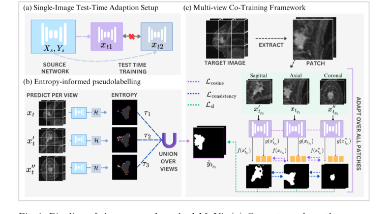Figure 1. Pipeline of the proposed method MuVi. (a) Our setup where the source network is adapted independently for each target sample xt, (b) computing pseu- dolabel through entropy-threshold union of prediction from each view, (c) Adap- tation via patch-based training through our multi-view consistency framework

Tearing the Equations Apart

Let's break down every single gear and spring in this mathematical machinery.

In the Pseudolabel Equation ($\hat{y}$):
* $\hat{y}$: The master pseudolabel. This is the model's best, most confident guess of where the tumor is, which will act as the "ground truth" for the upcoming training phase.
* $v \in \{x_t, x'_t, x''_t\}$: The three distinct 3D views of the target image (axial, coronal, and sagittal planes).
* $j$: A specific voxel (a 3D pixel) in the MRI scan.
* $f(v(j))$: The neural network's raw prediction for that specific voxel.
* $\sigma(\cdot)$: The sigmoid activation function. It squashes the raw prediction into a probability between 0 and 1.
* $H(\cdot)$: The Shannon Entropy function, defined as $H(z) = -z \log_2(z) - (1-z) \log_2(1-z)$. Logically, this acts as a strict bouncer. If the model is unsure (e.g., predicting a 50% chance of a tumor), the entropy is high. If it is highly confident (e.g., 99% or 1%), the entropy is low.
* $\tau_v$: The confidence threshold. If the entropy is below this number, the prediction is accepted.
* $\bigcup$: The Union operator. Why use a union instead of an intersection? Because different 3D views capture different anatomical boundaries. An intersection would only keep voxels that all three views agree on, resulting in a severely shrunken, conservative tumor mask. A union aggregates the highly confident discoveries from all perspectives, building a comprehensive 3D map.

In the Self-Learning Equation ($\mathcal{L}_{sl}$):
* $\sum$: Summation over the three views. Why addition instead of multiplication? We want the total penalty to be the accumulated errors from all perspectives. If we multiplied them, a near-zero error in one view would cancel out massive errors in another, which is dangerous in medical imaging.
* $\mathcal{L}_{DICE}$: The Dice Loss. It measures the spatial overlap between the prediction and the pseudolabel. It acts as a rubber band, pulling the global shape of the predicted tumor to match the pseudolabel, which is crucial for highly imbalanced medical images where the tumor is tiny compared to the background.
* $\mathcal{L}_{CE}$: Cross-Entropy Loss. It evaluates voxel-by-voxel classification accuracy. Why add DICE and CE together? DICE is excellent for global shape but can be mathematically unstable during gradient descent. CE is highly stable but ignores global structure. Adding them provides a perfectly balanced, stable gradient.

In the Feature Consistency Equation ($\mathcal{L}_{cosine}$):
* $g(\cdot)$: The feature extractor (the deep internal layers of the neural network, before the final classification).
* $\cos(\cdot, \cdot)$: Cosine similarity.
* $1 - \cos(\cdot, \cdot)$: Cosine distance. Why use cosine distance instead of standard L2 (Euclidean) distance? In deep, high-dimensional neural networks, the direction of a feature vector holds the semantic meaning (e.g., "this texture is a tumor"), while the magnitude just represents the intensity of that feature. Cosine distance strictly measures the angle between vectors, forcing the network to align the semantic meaning of the tumor regardless of the viewing angle.

In the Total Loss ($\mathcal{L}_{total}$):
* $\lambda_1, \lambda_2, \lambda_3$: Scalar weights that calibrate the importance of the self-learning, prediction consistency, and feature consistency. The authors set these equally to balance the forces.

Step-by-Step Flow: The Assembly Line

Let's trace a single abstract data point—a 3D MRI scan of a patient—through this engine.

1. Slicing the Perspectives: The 3D scan $x_t$ enters the system and is immediately permuted into three distinct geometric orientations: axial, coronal, and sagittal.
2. The Confidence Filter: The frozen model looks at all three views and generates preliminary tumor masks. The Entropy function $H$ scans every single voxel. If the model hesitates or outputs a weak probability, that voxel is instantly discarded.
3. Forging the Master Key: The surviving, highly confident voxels from all three views are fused together via the Union operator $\bigcup$ to create the Golden Pseudolabel $\hat{y}$.
4. Patch Extraction: Because 3D medical images are massive and would crash the GPU memory, the image is chopped into smaller 3D blocks (patches) $x_{t_{p_i}}$.
5. The Dual-Correction Loop: Each patch passes through the network. The network's final output is compared against the Golden Pseudolabel using the DICE + CE loss. Simultaneously, the deep internal represntation of the patch $g(x)$ is extracted. The Cosine loss grabs the feature vectors from the different views and physically rotates them in high-dimensional space until they point in the exact same direction.

Optimization Dynamics: How It Actually Learns

This is where the authors pull off a brilliant optimization stragety. How do you train a model on a single image without it instantly overfitting and collapsing?

The model updates in a single epoch. Furthermore, the authors do not update the entire network. They freeze almost everything and only allow the gradients to update the affine parameters ($\gamma$ and $\beta$) of the Normalization layers.

Why? In standard Batch Normalization, the network relies on the mean ($\mu$) and variance ($\sigma$) of a large batch of images. But here, we only have one image. A single image does not have enough statistical power to redefine the entire dataset's distribution. Therefore, the authors lock the original source domain's $\mu$ and $\sigma$ in place.

As the gradients flow backward from $\mathcal{L}_{total}$, they only tweak $\gamma$ (scale) and $\beta$ (shift). This acts as a lightweight calibration knob. It shifts and scales the feature maps just enough to adapt to the new hospital's MRI contrast and brightness, without destroying the fundamental tumor-detecting logic the model learned originally.

The loss landscape here is heavily constrained by the multi-view consistency. By forcing the model to agree with itself across different geometric transformations, the $\mathcal{L}_{cosine}$ and $\mathcal{L}_{consistency}$ terms act as massive regularizers. They carve a steep, narrow path to convergence, preventing the model from hallucinating wild predictions based on a single noisy image. The network rapidly settles into a local minimum that perfectly bridges the gap between the old training data and the new, unseen patient.

Results, Limitations & Conclusion

Imagine you learn to drive in a quiet, sunny suburban town. You master the roads, the signs, and the flow of traffic. Now, suddenly, you are dropped into the middle of a chaotic, blizzard-struck metropolis and told to drive. Your fundamental driving skills are intact, but the domain has shifted so drastically that you are bound to make mistakes.

In the world of medical imaging, deep learning models face this exact nightmare. A model trained on images from one hospital's MRI scanner will often fail catastrophically when analyzing images from a different hospital's scanner. The magnetic field strength, the reconstruction software, and the imaging protocols create a "domain shift."

To fix this, researchers use Test-Time Adaptation (TTA). Instead of retraining the entire model from scratch—which is as expensive as buying a new \$150,000 medical device every time you switch hospitals—TTA tweaks the model slightly right at the moment it is making a prediction. However, existing TTA methods have a fatal flaw: they require a large batch of images to understand the new enviornment. In a real clinical setting, doctors don't have batches; they have a single 3D scan of a single patient waiting for a diagnosis. Furthermore, existing methods often treat 3D medical images like a stack of flat 2D photographs, completely ignoring the rich, volumetric reality of human anatomy.

This paper introduces a brilliant, source-free solution: Patch-Based Multi-View Co-Training (MuVi). Let's break down exactly how they solved this single-image 3D adaptation problem.

The Mathematical Core of the Problem and Solution

The Problem:
We are given a model $M(\theta_s)$ with parameters $\theta_s$ that has already learned a mapping function $f: X_s \rightarrow Y_s$ on a source dataset $s$. Our goal is to adapt this model to a new target domain $t$ to learn a new function $k: X_t \rightarrow Y_t$. The massive constraint here is that we have no access to the original source data, no access to the ground truth labels of the target data, and we must do this using only a single target image $x_t \in X_t$.

The Solution:
The authors tackle this through a combination of clever statistical preservation and geometric consistency.

1. Preserving Source Statistics:
   Standard Batch Normalization (BN) relies on the mean $\mu$ and variance $\sigma$ of a batch of data. If you try to calculate $\mu$ and $\sigma$ from a single image, the math breaks down into noisy chaos. Therefore, the authors freeze the original source statistics $\mu_s$ and $\sigma_s$. They only allow the network to update the learnable affine transformation parameters $\gamma$ and $\beta$ during test time, where the normalized output is $y = \gamma \hat{x} + \beta$.

2. Multi-View Co-Training & Entropy-Guided Self-Training:
   Since they only have one 3D image, they extract overlapping 3D patches $\{x_{t_{p_1}}, x_{t_{p_2}}, \dots, x_{t_{p_n}}\}$. For each patch, they mathematically permute the axes to look at it from three different anatomical planes: axial, sagittal, and coronal. Let's define these three views as $v \in \{x_{t_{p_i}}, x'_{t_{p_i}}, x''_{t_{p_i}}\}$.

To train the model without human labels, they force the model to generate its own "pseuodolabels." They calculate the pixel-wise Shannon entropy to measure the model's uncertainty:
$$H(z) = -z \log_2(z) - (1-z) \log_2(1-z)$$
where $z \in [0, 1]$ is the predicted probability of a tumor. They only accept predictions where the entropy $H(z)$ is below a strict threshold $\tau$. The final pseudolabel $\hat{y}$ is the union of the confident predictions across all three views.

1. The Optimization Objective:
   The model is then adapted for just a single epoch by minimizing a tripartite loss function:
   $$\mathcal{L}_{total} = \lambda_1 \mathcal{L}_{sl} + \lambda_2 \mathcal{L}_{consistency} + \lambda_3 \mathcal{L}_{cosine}$$
   Here, $\mathcal{L}_{sl}$ forces the model's predictions to match the high-confidence pseudolabels using Dice and Cross-Entropy loss. $\mathcal{L}_{consistency}$ forces the predictions from the three different views to agree with each other. Finally, $\mathcal{L}_{cosine}$ operates deep inside the neural network, forcing the feature extractor $g(\cdot)$ to align the deep embeddings of the different views using cosine similarity:
   $$\mathcal{L}_{cosine} = 1 - \cos(g(x_{t_{p_i}}), g(x'_{t_{p_i}})) + 1 - \cos(g(x_{t_{p_i}}), g(x''_{t_{p_i}}))$$

The Experimental Architecture and the "Victims"

The authors didn't just claim their math worked; they engineered a ruthless experimental architecure to prove it. They trained a baseline 3D UNet on a massive dataset (Duke-Breast-Cancer-MRI) and then ambushed it with two completely unseen datasets (TCGA-BRCA and ISPY1) featuring different scanners (GE, Siemens, Philips) and different acquisition planes.

The "victims" in this experiment were state-of-the-art TTA methods: PTN, Tent, BNAdapt, InTent, and MEMO.

The definitive evidence of MuVi's superiority was stark. Methods like Tent and PTN, which try to update batch statistics based on a single image, actually degraded the baseline model's performance. They fell into the trap of single-image statistical noise. MEMO, which uses augmentations, barely moved the needle. MuVi, however, achieved a massive leap, improving the Dice Similarity Coefficient by up to 5.57% over the baseline.

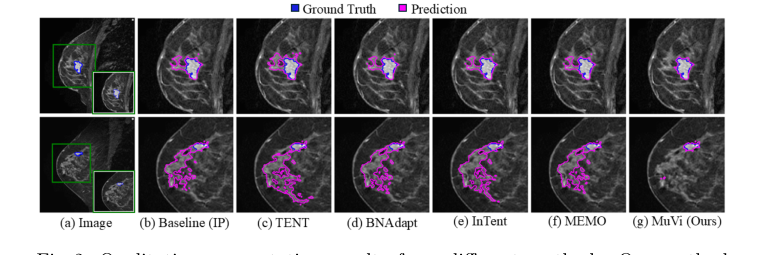Figure 2. Qualitative segmentation results from different methods. Our method localizes the tumor precisely while removing the misidentified breast tissue

The smoking gun was their ablation study. When they removed the multi-view consistency constraint, or when they discarded the source BN statistics, the model's performance collapsed. This proved undeniably that their specific mechanism—forcing a 3D model to agree with itself across different anatomical planes while anchored by source statistics—was the exact reason it succeeded in reality. Interestingly, when they swapped Batch Normalization for Instance Normalization, their unsupervised method achieved distance error metrics even lower than a model fully supervised on the target data. To be honest, I'm not completely sure how an unsupervised adaptation beats a supervised upper bound in that specific metric, but it strongly suggests that Instance Normalization is vastly superior at handling single-patient style variations.

Discussion Topics for Future Evolution

Based on these brilliant findings, here are several avenues for future exploration to stimulate critical thinking:

• The Limits of Single-Instance Adaptation: While adapting to a single image is clinically ideal, does it inherently sacrifice the "wisdom of the crowd"? If a model hyper-adapts to one patient's unique anatomy, does it risk hallucinating tumors out of benign anomalies that a population-level statistical view would have ignored? How can we balance single-patient personalization with global anatomical priors?
• Beyond Entropy for Uncertainty Quantification: The authors use Shannon entropy as a proxy for model confidence. However, deep neural networks are notoriously overconfident, often yielding low entropy even when they are completely wrong. Could we integrate Bayesian Neural Networks or Evidential Deep Learning to generate mathematically rigorous uncertainty bounds, thereby creating much safer and more accurate pseudolabels?
• Cross-Modality Geometric Consistency: This paper proves that multi-view consistency works when shifting between different MRI scanners. But what if the domain shift is across entirely different physical modalities, such as adapting an MRI-trained model to a CT scan? The underlying 3D geometry of the organs remains the same, but the pixel intensity physics are entirely different. Could $\mathcal{L}_{cosine}$ be evolved to align structural features across modalities without relying on pixel-level similarities?

Isomorphisms with other fields

A self-calibrating mechanism that optimizes a predictive function on a single unlabled high-dimensional tensor by enforcing logical consensus across its orthogonal geometric projections.

Target Field 1: Astrophysics and Black Hole Interferometry
In the realm of radio astronomy, particularly when imaging black holes using Very Long Baseline Interferometry (VLBI), scientists face a massive "domain shift" problem. They receive sparse, noisy radio wave data from multiple telescopes scattered across the Earth. There is no "ground truth" image of a black hole to train their reconstruction models on. The core logic of this paper is a perfect mirror image of the VLBI problem: just as this paper extracts axial, sagittal, and coronal views from a single MRI to force a model to agree with itself, astrophysicists force their image reconstruction models to find a single 3D spatial geometry that perfectly satisfies the partial, 2D frequency-domain projections captured by different telescopes. Both fields solve the problem of "zero ground truth" by substituting it with "multi-view consistency."

Target Field 2: High-Frequency Financial Arbitrage
In quantitative finance, an algoritm must constantly evaluate the "true" price of a complex derivative. However, in highly volatile markets, the historical training data (source domain) becomes instantly obsolete during a market crash (domain shift). The paper's logic mirrors statistical arbitrage. Imagine a single asset traded simultaneously across three different global exchanges (the "three views"). The algorithm doesn't know the absolute true fundamental value of the asset (no ground truth labels), but it knows that the price across all three exchanges must mathematically align. By minimizing the pricing divergence between these exchanges—much like minimizing the $\mathcal{L}_{consistency}$ and $\mathcal{L}_{cosine}$ losses between image patches—the financial model can self-adapt its internal parameters in real-time to the new market regime using only a single moment of data.

The "What If" Scenario
What if a geophysicist working on real-time earthquake early warning systems "stole" this exact equation tomorrow? Currently, seismic models struggle when an earthquake occurs in a novel geological domain (a previously dormant fault line) because the rock density and wave propagation characteristics differ entirely from the training data. If the researcher applied this paper's exact multi-view co-training equation, they could treat a single, unfolding seismic event as the "single test image." By taking the P-waves, S-waves, and surface waves as the three orthogonal "views," the model could calculate an entropy-weighted pseudolabel of the fault rupture. By minimizing the loss function $$\mathcal{L}_{total} = \lambda_1\mathcal{L}_{sl} + \lambda_2\mathcal{L}_{consistency} + \lambda_3\mathcal{L}_{cosine}$$ across these seismic wave projections, the early warning system would self-calibrate in a fraction of a second. The breakthrough would be the ability to accurately predict the magnitude and spatial segmentation of an earthquake's epicenter in a completely unmapped geological zone, using only the very first milliseconds of the anomalous wave itself.

This paper enriches the Universal Library of Structures by mathematically proving that absolute truth is not strictly necessary for calibration, provided one can enforce rigorous internal consistency across multiple orthogonal perspecives of the exact same reality.

---