Temporal Atlas-Guided Generation of Longitudinal Data via Geometric Latent Embeddings
This paper introduces a new AI model that creates realistic "time lapse" medical images from static scans, helping us understand how body parts grow and change.
Background & Academic Lineage
To understand the roots of this research, we have to look at the historical evolution of medical imaging. Decades ago, medical scans like CTs or MRIs were treated as static photographs—a single snapshot of a patient's internal anatomy at one specific moment. However, doctors and researchers quickly realized that human anatomy is not static; it is a highly dynamic process driven by genetics, nutrition, and disease. To accurately diagnose conditions like Alzheimer's or track the normal developement of a child's skeletal structure, the medical field needed to shift from 3D static images to 4D statistical shape analysis. This meant adding "time" as the fourth dimension. The clinical need to observe the "movie" of a patient's anatomy rather than just a "photograph" gave birth to the demand for longitudinal imaging data.
However, the fundamental limitation that forced the authors to write this paper is a severe data bottleneck. Capturing true longitudinal data requires scanning the exact same patient repeatedly over months or years. This is incredibly expensive (often costing thousands of dollars, e.g., \$1,000+ per scan), time-consuming, and logistically difficult, leading to a massive shortage of this data. Previous AI models attempted to generate synthetic longitudinal data, but they suffered from a fatal flaw: they required massive datasets of existing longitudinal data just to train the algorithms. Meanwhile, hospitals are sitting on mountains of "cross-sectional" data (single scans from many different people). Previous methods could not effectively use this abundant cross-sectional data to predict individual, subject-specific changes over time.
To bridge this gap, the authors introduce a few highly specialized concepts. Here is what they mean in everyday terms:
- Longitudinal Data: Imagine a time-lapse video of a single plant growing from a sprout into a blooming flower. It tracks the exact same subject over time, showing cause-and-effect in its growth.
- Cross-sectional Data: Imagine taking a single group photo of a kindergarten class, a middle school class, and a high school class. You can see what an "average" 5-year-old or 15-year-old looks like, but you have no idea how one specific kindergartener will look when they reach high school.
- Atlas Building: Think of this as creating a "composite sketch." If you take thousands of photos of different 10-year-old hips and mathematically blend them together, you get a standard, average template (the atlas) that represents a typical 10-year-old hip.
- Diffeomorphism: Imagine printing a medical image on a sheet of highly stretchable, magical rubber. You can stretch, warp, and twist this rubber to make one shape look like another, but you are never allowed to tear the rubber or fold it over itself. Because it's never torn, you can always perfectly reverse the stretching to get back to the original shape.
- Latent Embeddings: Imagine trying to describe a complex 3D car to a friend over the phone. Instead of describing every single bolt, you just give them a few key numbers: length, weight, and engine size. A latent represntation is the AI's way of compressing a complex 3D medical image into a short list of essential mathematical features.
Mathematically, the authors solved the problem of generating subject-specific longitudinal data using mostly cross-sectional data. They did this by forcing two separate AI tasks to work together: building an average atlas for each age group, and learning how to warp shapes across different ages.
First, they define the problem of building an atlas by minimizing an energy function:
$$E(I, v_0^n) = \sum_{n=1}^N \frac{1}{\sigma^2} \text{Dist}[I \circ \phi_1^{-1}(v_0^n), I_n] + \text{Reg}(v_0^n)$$
In plain English, this equation tries to find a perfect average image ($I$) by measuring the distance ($\text{Dist}$) between the warped average image and the actual patient images ($I_n$). The $\text{Reg}$ term is a rule that ensures the "stretching of the rubber" remains smooth and realistic.
To achive their ultimate goal, the authors designed a unified neural network that minimizes a combined total loss function:
$$\ell = \mathcal{L}_{\text{tempo-atlas}}(\Theta) + \mathcal{L}_{\text{longitudinal}}(\Psi) + \gamma \mathcal{L}_{\text{latent}}(\mathbf{Z})$$
Here, the model is penalized if it fails at three things simultaneously:
1. $\mathcal{L}_{\text{tempo-atlas}}$: It must build accurate average atlases for each specific age group.
2. $\mathcal{L}_{\text{longitudinal}}$: It must accurately figure out how to warp an atlas from one age (e.g., age 10) to the next age (e.g., age 12).
3. $\mathcal{L}_{\text{latent}}$: It must ensure that the compressed mathematical summaries (embeddings) of these shapes cluster together logically, meaning shapes that look biologically similar are kept close together in the AI's "brain."
By solving this joint equation, the AI learns the general rules of aging from the population (the atlases) and applies those rules to a single snapshot of a new patient, successfully predicting how that specific patient's anatomy will grow over time.
| Notation | Description |
|---|---|
| $I_n$ | The $n$-th input image in a dataset (e.g., a specific patient's CT scan). |
| $I$ | The mean or template image, representing the "average" anatomy (the Atlas). |
| $\phi$ | The mathematical transformation (the "warping" function) applied to an image. |
| $v_0$ | The initial velocity field, which dictates how the shape will start deforming. |
| $\sigma^2$ | The noise variance in the images, used to weight the distance measurement. |
| $A_q$ | The specific anatomical atlas constructed for a given age/time $q$. |
| $\Theta$ | The learnable parameters of the neural network responsible for building the temporal atlases. |
| $\Psi$ | The learnable parameters of the neural network responsible for cross-age (longitudinal) registration. |
| $\mathbf{z}_q^i$ | The latent embedding (compressed mathematical representation) of an image at age $q$. |
| $\gamma$ | A tuning parameter that controls how strongly the model enforces the latent embedding rules. |
Problem Definition & Constraints
Imagine you are tasked with creating a time-lapse video of a specific child growing up. However, instead of having a continuous video of that one child, you are handed a massive photo album containing pictures of different children at various ages. You can easily figure out what an average 5-year-old or an average 10-year-old looks like. But predicting exactly how one specific 5-year-old will look at age 10 is incredibly hard because we lack the anotomical history of that specific child.
This is the exact scenario medical researchers face when trying to model how human organs and bones develop over time.
The Starting Point and The Goal State
The Input (Current State): The medical field is rich with 3D cross-sectional imaging data. These are single-timepoint snapshots (like CT or MRI scans) taken from multiple different individuals. While abundant, these datasets represnt only a snapshot in time, offering zero information about cause-and-effect biological changes.
The Output (Goal State): Clinicians desperately need 4D longitudinal data. This means having subject-specific, time-varying structural changes of the same patient over time. If a doctor inputs a 3D scan of an 8-year-old patient's hip, the goal is to output a biologically accurate, highly personalized 3D scan of what that exact patient's hip will look like at age 10 or 15.
The Mathematical Gap: The missing link is a continuous, invertible transformation field that can evolve a specific anatomical structure forward in time without relying on paired longitudinal training data. We need a mathematical bridge that connects a population-level average (an "atlas") to a subject-specific temporal trajectory.
The Painful Dilemma
To generate realistic longitudinal data, deep learning models (like sequence-aware diffusion models) typically require massive amounts of ground-truth longitudinal data to train on. Herein lies the trap:
You cannot train a good longitudinal model without longitudinal data, but longitudinal data is notoriously expensive (often costing upwards of \$1000 per patient scan), time-consuming, and incredibly difficult to collect. If researchers try to bypass this by training models solely on the abundant cross-sectional data, the generated future images lose their subject-specific fidelity. The model ends up predicting a generic "average" person rather than preserving the unique skeletal geometry of the original patient. Previous researchers have been trapped in this painful trade-off between data availability and temporal accuracy.
The Harsh Walls and Constraints
To solve this, the authors hit several brutal constraints:
- Extreme Data Sparsity: Real longitudinal data takes years to collect. Patients drop out of studies, imaging hardware changes, and aligning scans taken years apart introduces massive variability.
- The Physics of Biological Deformation: Bone and tissue growth isn't just a simple pixel shift; it involves complex, non-linear biological changes. To model this, the authors had to use Large Deformation Diffeomorphic Metric Mapping (LDDMM). This ensures that the transformations are smooth and invertible (diffeomorphic)—meaning tissues don't magically tear, cross over, or fold into themselves. However, calculating this requires integrating velocity fields forward in time using the Euler-Poincaré differential (EPDiff) equation:
$$ \frac{\partial v_t}{\partial t} = -K \left[ (D v_t)^T \cdot m_t + D m_t \cdot v_t + m_t \cdot \text{div} \, v_t \right] $$
Solving this to find the optimal velocity fields ($v_t$) and momentum vectors ($m_t$) is a massive computional burden. - The Blurry Artifact Wall: When previous state-of-the-art models (like VoxelMorph or B-splines) attempted to morph anatomies across large age gaps, they introduced severe distortions and blurry boundaries. Preserving fine anatomical details, like the tri-radiate cartilages in a developing hip, is exceptionally difficult when the model is forced to guess how a structure expands over years.
How They Solved It: A Unified Mathematical Framework
The authors realized that to break out of the dilemma, they couldn't just build a generator; they had to simultaneously build a map. They designed a novel deep learning framework that jointly performs two tasks: Temporal Atlas Building (finding the population average at a given age) and Cross-age Image Registration (aligning that average to specific targets to model growth).
First, they define a loss function to construct a sequence of age-specific atlases ($A_q$) by minimizing the distance between the atlas and the cross-sectional images ($I_i^q$), regularized by the velocity field ($v_i^q$):
$$ \mathcal{L}_{\text{tempo-atlas}}(\Theta) = \sum_{q=1}^{Q} \sum_{i=1}^{N_q} \text{Dist}\left[ \phi_{q \to i}^{-1}(\Theta) \circ A_q, I_i^q \right] + \text{Reg}(v_i^q) $$
Next, they model the longitudinal changes by aligning the source atlas to target ages ($q'$):
$$ \mathcal{L}_{\text{longitudinal}}(\Psi) = \sum_{m=1}^{M} \text{Dist}\left[ \phi_{q \to q'}^{-1}(\Psi) \circ A_q, I_{q'}^m \right] + \text{Reg}(v_{m}^{q'}) $$
The Breakthrough: The true genius of the paper is how they tie these two spaces together using Distinctive Latent Embeddings. They force the neural network to learn a latent space $\mathbf{Z}$ where anatomically similar structures cluster tightly together, while the distance between these embeddings strictly correlates with the physical deformation (the velocity fields) required to morph between them.
They enforce this with a specialized loss function:
$$ \mathcal{L}_{\text{latent}}(\mathbf{Z}) = \mathbb{E} \left[ -\log(\sigma(\text{sim}(\mathbf{z}_q^i, \mathbf{z}_{q'}^m))) \right] + \lambda \mathbb{E} \left[ \text{Corr}\left( \|\mathbf{z}_q^i - \mathbf{z}_{q'}^m\|^2, \|v_q^i - v_{q'}^m\|^2 \right) \right] $$
The first term uses cosine similarity to group related shapes. The second term is the masterstroke: it calculates the correlation between the Euclidean distance of the latent embeddings ($\|\mathbf{z}_q^i - \mathbf{z}_{q'}^m\|^2$) and the physical energy of the deformation ($\|v_q^i - v_{q'}^m\|^2$).
By mathematically locking the abstract latent space to the physical laws of diffeomorphic deformation, the model can look at a single cross-sectional scan, map it to the temporal atlas, and accurately project how that specific geometry will evolve over time—completely bypassing the need for massive longitudinal training datasets.
Why This Approach
To understand why the authors chose this highly specific, mathematically dense approach, we first have to look at the exact moment traditional state-of-the-art (SOTA) methods hit a brick wall.
In recent years, the deep learning community has been obsessed with generative models. If you want to generate a sequence of images showing how a child's hip bone grows over time, your first instinct might be to use a Diffusion model or a Transformer. In fact, the authors explicitly point out that previous researchers have tried exactly this: Yoon et al. used sequence-aware diffusion models, and Puglisi et al. used latent diffusion models to simulate structural changes over time.
But here is the fatal flaw that forced the authors to abandon these popular approaches: standard generative models are incredibly data-hungry. They require massive, paired longitudinal datasets—meaning you need thousands of 3D scans of the same patients taken year after year. In a real-world clinical enviornment, this type of data is prohibitively expensive, time-consuming, and practically non-existent. The vast majority of available medical data is cross-sectional (snapshots of different people at single, isolated moments in time). Diffusion models and GANs simply cannot learn subject-specific temporal dynamics without seeing the actual temporal sequence during training. They would fail here because they cannot hallucinate biologically accurate growth trajectories from disconnected snapshots.
Faced with this harsh constraint, the authors realized that the only viable solution was to embed the strict laws of physics and geometry into the learning process. They turned to Large Deformation Diffeomorphic Metric Mapping (LDDMM).
Why is this mathematically superior? A diffeomorphic transformation guarantees that the mapping between two anatomical shapes is smooth, continuous, and strictly invertible. In biology, tissues stretch and grow, but they do not randomly tear, fold onto themselves, or teleport. By framing the problem through the Euler-Poincaré differential (EPDiff) equation, the authors ensure that the geodesic path of anatomical growth is uniquely determined by integrating an initial velocity field $v_0$ forward in time:
$$ \frac{\partial v_t}{\partial t} = -K \left[ (D v_t)^T \cdot m_t + D m_t \cdot v_t + m_t \cdot \text{div} \, v_t \right] $$
This creates a perfect "marriage" between the problem's harsh constraints (lack of longitudinal data) and the solution's unique properties. Instead of trying to blindly guess how a bone grows, the model jointly performs two tasks: it builds an "atlas" (the average shape of a population at a specific age, say, 8 years old) and then learns the diffeomorphic velocity fields that warp the 8-year-old atlas into a 10-year-old atlas. It then applies these learned, biologically plausible velocity fields to a specific patient's baseline scan to generate highly realiable predictions of their future anatomy.
The structual advantage of this method over previous gold standards—like VoxelMorph (VM) or B-spline registration—is profound. Traditional registration methods just try to minimize pixel-wise differences between Image A and Image B. As shown in the paper's benchmarking, this often results in blurry boundaries and severe artifacts (like the distortions seen around the iliac crest in the VoxelMorph baseline).
To overcome this, the authors introduced a brilliant "Distinctive Latent Embedding" loss. They don't just align images; they force the neural network's latent space to perfectly mirror the physical deformation space. The loss function includes a term that measures the correlation between the distance of the latent embeddings $\mathbf{z}$ and the physical distance of the velocity fields $v$:
$$ \mathcal{L}_{\text{latent}}(\mathbf{Z}) = \dots + \lambda \mathbb{E}_{(\mathbf{z}_q^i, \mathbf{z}_{q'}^m)} \left[ \text{Corr} \left( \|\mathbf{z}_q^i - \mathbf{z}_{q'}^m\|^2, \|v_q^i - v_{q'}^m\|^2 \right) \right] $$
This mathematically forces the latent space to preserve the geometric and temporal relationships dictated by the velocity fields. It disentangles progressive shape variations across time, allowing the model to generate razor-sharp, artifact-free boundaries around complex growth centers like the tri-radiate cartilages.
To be honest, I'm not completely sure if this specific architecture reduces the computational memory complexity from $O(N^2)$ to $O(N)$, as the authors do not explicitly provide a Big-O algorithmic breakdown in the text. However, what is overwhelmingly clear is its data efficiency. By leveraging geometric latent spaces of diffeomorphisms, this framework achieves what SOTA Diffusion models cannot: it synthesizes highly accurate, subject-specific 4D longitudinal data using only sparse, cross-sectional 3D inputs.
Mathematical & Logical Mechanism
To understand the gravity of this paper, we first need to understand the fundamental data problem in medical imaging. Imagine trying to understand how a child grows by looking at a photo album. If you have a "longitudinal" album—photos of the same child taken every year—you can easily see the exact trajectory of their growth. But in the medical field, getting longitudinal 3D scans (like CT or MRI) of the same patient over many years is incredibly expensive, time-consuming, and rare. Instead, hospitals have mountains of "cross-sectional" data: single snapshots of different people at different ages.
The authors of this paper built a brilliant mathematical engine that takes these disconnected snapshots of different people and learns the underlying "rules of growth." It then uses these rules to generate a highly accurate, personalized 3D time-lapse (longitudinal data) for a brand new patient, predicting exactly how their anatomy will change over time.
Here is the exact mathematical machinery that makes this possible.
The Master Equations
The core engine of this paper is driven by a unified objective function that balances three massive tasks simultaneously: building an "average" template (atlas), predicting growth across ages, and forcing the model to understand the physical reality of these changes.
The total loss function that powers the entire network is:
$$ \ell = \mathcal{L}_{\text{tempo-atlas}}(\Theta) + \mathcal{L}_{\text{longitudinal}}(\Psi) + \gamma \mathcal{L}_{\text{latent}}(\mathbf{Z}) $$
But the true secret sauce—the most innovative part of this paper—is the Distinctive Latent Embedding loss, which acts as the brain of the operation:
$$ \mathcal{L}_{\text{latent}}(\mathbf{Z}) = \mathbb{E}_{(\mathbf{z}_q^i, \mathbf{z}_{q'}^m)} \big[ -\log(\sigma(\text{sim}(\mathbf{z}_q^i, \mathbf{z}_{q'}^m))) \big] + \lambda \, \mathbb{E}_{(\mathbf{z}_q^i, \mathbf{z}_{q'}^m)} \big[ \text{Corr} \big( \|\mathbf{z}_q^i - \mathbf{z}_{q'}^m\|^2, \; \|v_q^i - v_{q'}^m\|^2 \big) \big] $$
Tearing the Equations Apart
Let's dissect every single gear and spring in this mechanism.
From the Total Loss ($\ell$):
* $\ell$: The total loss. This is the ultimate "error score" the machine tries to minimize to zero.
* $\mathcal{L}_{\text{tempo-atlas}}(\Theta)$: The Temporal Atlas Building loss. This term measures how well the network (with parameters $\Theta$) can create an "average" anatomical template for a specific age. It acts as the baseline anchor.
* $\mathcal{L}_{\text{longitudinal}}(\Psi)$: The Cross-age Registration loss. This measures how well the network (with parameters $\Psi$) can warp an image from one age to match the anatomy of an older age. It is the "time machine" component.
* $\gamma$: A scalar weight (a balancing knob). It dictates how much attention the model should pay to the latent embeddings versus the image generation.
* Why addition instead of multiplication? The authors use addition to create a multi-task balancing scale. If they multiplied these terms, a near-zero score in the atlas loss would completely wipe out the gradients (the learning signals) for the longitudinal loss, halting the learning process entirely. Addition ensures that even if one task is performing perfectly, the model still feels the pressure to improve the others.
From the Latent Embedding Loss ($\mathcal{L}_{\text{latent}}(\mathbf{Z})$):
* $\mathbf{Z}$: The matrix of all latent embeddings. An embedding is a highly compressed, abstract mathematical summary of a 3D medical image.
* $\mathbb{E}_{(\mathbf{z}_q^i, \mathbf{z}_{q'}^m)}$: The expected value (average) over pairs of these compressed embeddings. $\mathbf{z}_q^i$ is the embedding of patient $i$ at age $q$, and $\mathbf{z}_{q'}^m$ is patient $m$ at age $q'$.
* Why an expectation instead of a hard summation ($\sum$)? In deep learning, calculating the exact sum of every possible pair of images across a massive dataset is computationally explosive. Using an expectation allows the model to stochastically sample random pairs during training, approximating the true average while saving massive amounts of memory.
* $-\log(\sigma(\dots))$: The negative log of a sigmoid function. This is a classic penalty mechanism. The sigmoid ($\sigma$) squashes values between 0 and 1 (like a probability). The negative log heavily penalizes the model if this value drops close to 0.
* $\text{sim}(\mathbf{z}_q^i, \mathbf{z}_{q'}^m)$: The cosine similarity between two embeddings. It measures the angle between two vectors.
* Logical Role: This entire first term acts as a gravitational pull. If two anatomical shapes are related, it forces their abstract mathematical vectors to point in the exact same direction in the latent space.
* $\lambda$: Another balancing knob, specifically controlling the strength of the physics constraint.
* $\text{Corr}(\dots)$: The Pearson correlation coefficient. It measures how linearly related two variables are.
* $\|\mathbf{z}_q^i - \mathbf{z}_{q'}^m\|^2$: The squared Euclidean distance between two abstract embeddings. Think of this as the "conceptual distance" between an 8-year-old hip and a 10-year-old hip.
* $\|v_q^i - v_{q'}^m\|^2$: The squared distance of their associated velocity fields ($v$). A velocity field is a 3D map of arrows dictating exactly how pixels must physically flow and stretch to morph one shape into another.
* Logical Role: This correlation term is pure genius. It acts as a strict physics inspector. It forces the abstract "conceptual distance" of the embeddings to perfectly correlate with the actual "physical stretching energy" required to deform the tissue. It prevents the neural network from cheating by placing images arbitrarily in the latent space.
Step-by-Step Flow
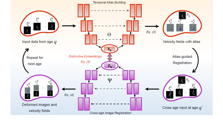 Figure 1. Overview of our model. Training: Our network constructs a sequence of tempo- ral atlases, starting at age q and modeling deformations across target ages. A geometric embedding loss in the latent space enforces structured, biologically meaningful anatom- ical evolution. Iterative refinement enhances the interplay between cross-sectional and longitudinal dynamics, generating anatomically coherent cross-age data. Inference: For each subject, we first align their baseline images to the corresponding age-specific atlas. The trained model Ψ operates as a longitudinal data generator, synthesizing anatomically plausible trajectories for unseen subjects by extracting geometric fea- tures through the atlas. It uses generated velocity fields from cross-age registration between age-specific atlases to deform subject-specific structures over time, ensuring a smooth and temporally consistent evolution
Let's trace a single abstract data point—a 3D CT scan of an 8-year-old patient's hip—as it moves through this mathematical assembly line.
- Compression: The raw 3D pixels of the 8-year-old hip enter the network and are immediately compressed into a dense, abstract vector $\mathbf{z}_q^i$.
- Anchoring: The system compares this vector to the "average 8-year-old hip" template it has built. It calculats how much the specific patient deviates from the norm.
- Time Travel: The user requests a prediction for what this hip will look like at age 12. The network looks at the "average 12-year-old" template. It generates a velocity field $v$—a fluid-like map of arrows that dictates how the 8-year-old bone must stretch, grow, and bend to reach the 12-year-old state.
- Quality Control: The $\mathcal{L}_{\text{latent}}$ loss kicks in. It checks the abstract distance between the 8-year-old vector and the 12-year-old vector. It strickly verifies that this abstract distance matches the physical energy of the velocity field $v$. If the math doesn't align with the physics, the model is penalized.
- Generation: Finally, the velocity field is applied to the original 3D scan, smoothly warping the pixels like a piece of digital clay to output a biologically accurate, synthetic 12-year-old hip scan.
Optimization Dynamics
How does this complex architecure actually learn and converge?
The model optimizes its parameters using Gradient Descent (specifically the Adam optimizer). Initially, the loss landscape is highly chaotic. The network tries to take shortcuts, perhaps just blurring the 8-year-old image to make it look vaguely like a 12-year-old image to quickly reduce the image distance loss.
However, the model is constrained by diffeomorphic mathematics (specifically the Euler-Poincaré differential equations mentioned in the paper's background). This means the transformations must be smooth, continuous, and invertible—like folding a rubber sheet without ever tearing it or letting it pass through itself.
Because of this strict physical constraint, the loss landscape is shaped like a steep, smooth funnel. As the gradients flow backward through the network, the embeddings $\mathbf{Z}$ are forced to organize themselves beautifully. Scans of similar ages cluster tightly together, while scans of different ages space themselves out in exact proportion to the physical growth required to transition between them. Over 1000 epochs, the system reaches an equilibrium: the generated atlases become razor-sharp, and the predicted growth trajectories become anatomically flawless, allowing the model to hallucinate the future of a patient's anatomy with incredible precision.
Results, Limitations & Conclusion
The Core Problem: Escaping the Snapshot Trap
To understand the magnitude of this paper, we first need to understand the fundamental difference between two types of medical data: cross-sectional and longitudinal.
Imagine you want to understand how human faces age. If you take a photograph of 100 different people, each at a different age from 5 to 50, you have cross-sectional data. You can guess the general trend of aging, but you don't know exactly how the 5-year-old will look when they are 50. Now, imagine taking a photograph of the exact same person every single year from age 5 to 50. That is longitudinal data. It captures the true, subject-specific spatiotemproal dynamics of change.
In medical imaging, longitudinal 3D data (making it 4D data over time) is the holy grail for tracking how anatomical structures develop or how diseases progress. However, collecting this data is a logistical nightmare. It is incredibly expensive—often costing upwards of \$10,000 per patient in scan fees and administrative overhead across a decade—and highly prone to patient dropout. Consequently, the vast majority of medical databases are cross-sectional.
The authors of this paper faced a massive constraint: How do we accurately predict the future 3D anatomical shape of a specific patient when our training data mostly consists of disconnected snapshots of different people?
The Mathematical Engine: Diffeomorphisms and Latent Time-Travel
To solve this, the authors didn't just train a standard neural network to guess the next frame. They built a framework that jointly performs two tasks: Atlas Building (finding the "average" shape of a population at a specific age) and Longitudinal Data Generation (predicting how a specific subject's shape evolves across ages).
They grounded their solution in the mathematics of Large Deformation Diffeomorphic Metric Mapping (LDDMM). In simple terms, a diffeomorphism is a smooth, continuous, and invertible transformation. Imagine morphing a clay sculpture of a 5-year-old's hip bone into a 10-year-old's hip bone without ever tearing the clay or folding it onto itself.
The baseline energy function to build an atlas (a template image $I$) from a set of $N$ images is defined as:
$$E(I, v_0^n) = \sum_{n=1}^N \frac{1}{\sigma^2} \text{Dist}[I \circ \phi_1^{-1}(v_0^n), I_n] + \text{Reg}(v_0^n)$$
Here, $v_0^n$ represents the initial velocity field—the "push" needed to start morphing the template into the target image $I_n$. The transformation path is governed by the Euler-Poincaré differential (EPDiff) equation, which dictates how this velocity flows forward in time:
$$\frac{\partial v_t}{\partial t} = -K \left[ (D v_t)^T \cdot m_t + D m_t \cdot v_t + m_t \cdot \text{div} \, v_t \right]$$
To be honest, the paper doesn't explicitly detail the exact computational memory footprint required to solve this integration during deep learning training, but given the 3D nature of the data, we can infer it requires heavy GPU lifting (which they handled using an RTX A6000).
The true genius of their architecture lies in the Distinctive Latent Embeddings. They force the neural network to learn a latent space $\mathbf{Z}$ where the mathematical distance between two embeddings perfectly correlates with the physical deformation required to morph between them. Their latent loss function is:
$$\mathcal{L}_{\text{latent}}(\mathbf{Z}) = \mathbb{E}_{(\mathbf{z}_q^i, \mathbf{z}_{q'}^m)} \left[ -\log(\sigma(\text{sim}(\mathbf{z}_q^i, \mathbf{z}_{q'}^m))) \right] + \lambda \, \mathbb{E}_{(\mathbf{z}_q^i, \mathbf{z}_{q'}^m)} \left[ \text{Corr} \left( \|\mathbf{z}_q^i - \mathbf{z}_{q'}^m\|^2, \, \|v_q^i - v_{q'}^m\|^2 \right) \right]$$
The first term forces related shapes to cluster together using cosine similarity. The second term is the masterstroke: it ensures that the squared Euclidean distance between two latent vectors $\|\mathbf{z}_q^i - \mathbf{z}_{q'}^m\|^2$ correlates with the physical "effort" (the velocity field distance $\|v_q^i - v_{q'}^m\|^2$) needed to deform one shape into another.
The final objective function elegantly balances temporal atlas building, cross-age registration, and this latent embedding:
$$\ell = \mathcal{L}_{\text{tempo-atlas}}(\Theta) + \mathcal{L}_{\text{longitudinal}}(\Psi) + \gamma \mathcal{L}_{\text{latent}}(\mathbf{Z})$$
The Experiment: Ruthless Validation Against Reality
The authors didn't just throw metrics at a wall; they architected a highly rigorous experiment. They trained their model on a cross-sectional dataset of normal male hips (ages 4-18). But to prove their model actually worked, they tested it on a hidden, highly valuable dataset of true longitudinal CT scans (12 patients who actually had multiple scans years apart).
The Victims (Baselines):
For atlas building, they completely dismantled established models like B-spline, Multi-contrast registration (M-c. reg.), and VoxelMorph (VM). For longitudinal generation, they defeated NAHA (Nearest-Age Hip Approximation) and ABAA (Age-Based Atlas Approximation).
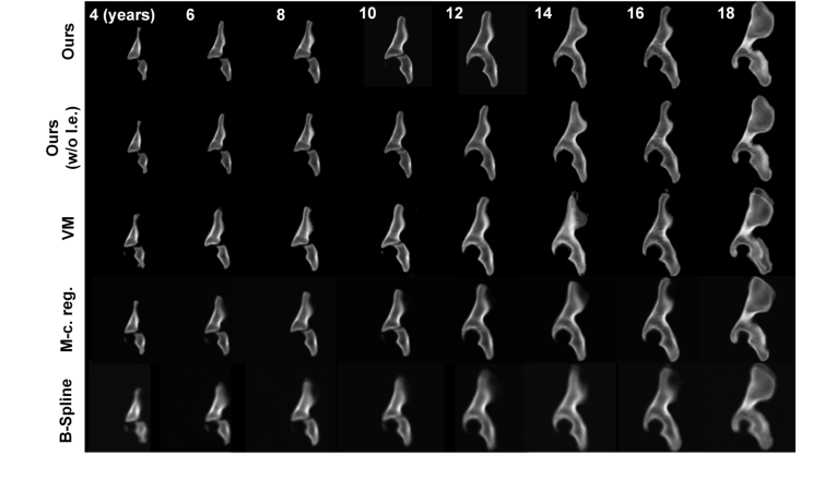 Figure 2. Comparison of our method with SOTA techniques for temporal hip atlas gener- ation. The age ranged from 4- to 18-years-old. Visually, our method achieved the best performance in atlas building, producing the sharpest boundaries around the growth centers of the hips (i.e., around the tri-radiate cartilages) and the margins of the hip bones (i.e., around the ilium and ischium) compared to other SOTA techniques
The Definitive Evidence:
The proof wasn't just in the Dice score (though they achieved a dominant 0.88). The undeniable evidence was visual and geometric. They took a real CT scan of a 12-year-old patient's hip, fed it into their model, and asked it to hallucinate the 15-year-old version of that exact same patient.
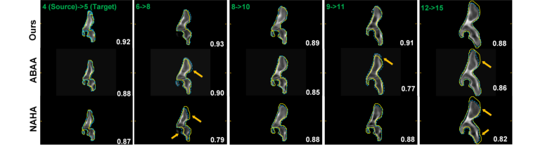 Figure 4. Comparison of various methods for the longitudinal data generation task based on a real longitudinal dataset. For example, in the first column, given an input hip dataset from a 4-year-old subject (source), the longitudinal data generator predicted the 3D synthetic longitudinal CT hip shape of the same subject at the age of 5. The source and target ages are denoted in green text in the left upper corner of each frame. The segmentation contour (blue dashed line) produced by our method aligns better with the ground truth contour (yellow line) than other techniques, as indicated by the higher Dice scores (white text). Arrows highlight regions with large alignment errors
When they overlaid their synthetic 15-year-old hip against the actual 15-year-old scan of that patient, the boundaries matched beautifully. The baselines failed miserably here—VoxelMorph created severe artifact distortions around the posterior iliac crest, and other methods produced blurry, anatomically impossible bone margins. The authors' model preserved the sharp, fine anatomical details around the tri-radiate cartilages, proving that their latent space had successfully learned the biological rules of bone growth, rather than just blindly interpolating pixels.
Future Trajectores and Discussion Topics
Based on the profound implications of this framework, here are several critical avenues for future exploration:
-
Integration of Biomechanical Physics Priors:
Currently, the model learns the rules of growth purely from geometric transformations (diffeomorphisms). However, bone development is heavily influenced by physical forces (Wolff's Law—bones adapt to the loads placed upon them). How could we inject biomechanical stress tensors into the EPDiff equation? If a child has an abnormal gait, could we condition the latent space to predict how that specific mechanical stress will alter their future bone shape? -
Branching Pathological Latent Spaces:
This paper focused on normal male hips to establish a baseline. But disease is rarely a linear progression. If we introduce pathological data (e.g., hip dysplasia), how do we structure the latent space so that a single cross-sectional scan can predict multiple possible futures? We need to discuss how to evolve this deterministic model into a probabilistic one, perhaps using diffusion models in the latent space to generate a "cone of uncertainty" for future disease progression. -
Cross-Modality Temporal Alignemnt:
The authors used CT scans, which provide excellent bone contrast but expose pediatric patients to ionizing radiation. The future of pediatric imaging is MRI or Ultrasound. However, these modalities have vastly different noise profiles and artifact behaviors. A fascinating discussion point is whether the geometric latent embeddings learned from CT data could be transferred to MRI data. Can the "velocity fields" of growth be decoupled from the pixel intensities of the imaging modality itself?
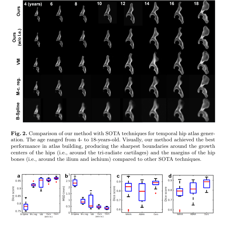 Figure 3. Boxplots of the atlas-to-patient (within-age) registration results based on the mean Dice score (a) and the MSD (b). Boxplots of the longitudinal data generation results for all testing cases (c) and for the cases when the age gap is >1 year (d) based on mean Dice score. The ages of the subjects in these experiments ranged from 4 to 18 years. Our method achieved superior performance compared to others