The Refining of Brain Connectivity Features on Residual Posterior Patterns
New AI model RP-LGN captures subtle connectivity changes for better disease diagnosis, outperforming others with improved accuracy & noise handling.
Background & Academic Lineage
To understand the true nature of the human brain, we must look beyond isolated regions and study how they communicate. Historically, neuroscientists used functional magnetic resonance imaging (fMRI) to capture brain activity. As the field of computational neuroscience evolved, researchers began representing the brain as a complex network, or a "graph," where brain regions are nodes and their communication pathways are edges. This naturally led to the adoption of Graph Neural Networks (GNNs) to diagnose neuropsychiatric disorders like Autism Spectrum Disorder (ASD) and ADHD by analyzing these functional connectivity patterns.
However, a critical bottleneck emerged. Traditional GNN approaches were fundamentally flawed for this specific task because they were focussing primarily on the brain regions themselves (the nodes) rather than the actual communication pathways (the edges). In neuropsychiatric disorders, the disease often manifests in the alteration of connections rather than the physical regions. Furthermore, previous models faced a massive computational hurdle: if you try to treat every single connection as a primary feature in a fully connected brain graph, the math explodes. A typical brain atlas might yield a matrix with billions of paramters, making it computationally impossible to process. On top of this, medical datasets are notoriously small and noisy, causing traditional models to overfit—meaning they memorize the training data but fail completely in real-world clinical applications.
To bridge this gap, the authors introduced the Residual-Posterior Line Graph Network (RP-LGN). Let's break down the highly specialized concepts they used into intuitive ideas:
Deconstructing the Jargon
- Functional Magnetic Resonance Imaging (fMRI) & BOLD Signal: In the paper, this is the raw data measuring blood flow changes in the brain.
- Everyday Analogy: Imagine a satellite tracking traffic congestion in a city at night by looking at the density of headlights. fMRI does this with blood flow; it tracks where the "traffic" (oxygenated blood) is moving to figure out which "intersections" (brain regions) are currently active and talking to each other.
- Line Graph Transformation: A mathematical technique to convert edges into nodes.
- Everyday Analogy: Suppose you are studying a global airline network. Normally, you study the cities (nodes) and draw lines for the flight routes (edges). A line graph transformation flips this: you make the flight routes the main subject of your study (the new nodes), and the cities just become the endpoints. This allows the AI to study the actual connections directly.
- Oversmoothing in GNNs: A phenomenon where passing messages between nodes too many times makes all nodes look identical.
- Everyday Analogy: Imagine mixing paint. If you gently swirl red and blue, you get a beautiful marbled pattern (useful information). But if you keep stirring relentlessly, you just end up with a flat, muddy purple. Oversmoothing is when the AI stirs the data too much, losing all the unique, distinguishing features of the brain.
- Bayesian Variational Posterior: A statistical method used in the model's final layer to quantify prediction uncertainty.
- Everyday Analogy: Instead of a weather app bluntly stating "It will rain tomorrow" (which might be wrong if the data is noisy), a Bayesian approach says, "I am 85% confident it will rain, give or take 5%." It calculates the margin of error, making the AI's medical diagnosis much more robust and trustworthy even when the patient's scan has a lot of background noise.
Mathematical Blueprint
To mathematically interpret how the authors solved this, we need to look at the variables that define their universe. They sparsify the initial connections using a $K$-Nearest Neighbors (KNN) approach to prevent the parameter explosion, and then map the graph to a line graph $\tilde{G}$. Finally, they optimize the model by maximizing the Evidence Lower Bound (ELBO), denoted as $\mathcal{L}_{VB}$.
| Notation | Description |
|---|---|
| $V$ | The set of nodes representing Regions of Interest (ROIs) in the brain. |
| $E$ | The set of edges representing functional connections between ROIs. |
| $G = (\mathbf{A}, \mathbf{X})$ | The original brain graph constructed from fMRI data. |
| $\mathbf{A} \in \mathbb{R}^{|V| \times |V|}$ | Adjacency matrix defining the partial correlation coefficients between brain regions. |
| $\mathbf{X} \in \mathbb{R}^{|V| \times |F|}$ | Node feature matrix based on Pearson correlation of pairwise BOLD signals. |
| $n$ | The total number of ROIs, where $|V| = n$. |
| $\mathcal{N}_i$ | The $K$ nearest neighbor nodes set of node $i$, used to sparsify the graph. |
| $\tilde{G} = \{\tilde{\mathbf{A}}, \tilde{\mathbf{X}}\}$ | The constructed line graph where original edges are now treated as nodes. |
| $\tilde{\mathbf{x}}_i$ | The feature vector of the $i$-th node in the newly constructed line graph. |
| $\tilde{\mathbf{Z}}^{(l)}$ | The output feature matrix of the $l$-th SAGEConv (GraphSAGE convolution) layer. |
| $W$ | The weight matrix of the final linear classification layer. |
| $\Sigma$ | The covariance matrix of the variational posterior, used to model uncertainty. |
| $\mathcal{L}_{VB}(\theta, \eta, \Sigma)$ | The variational lower bound (ELBO) used as the objective function to optimize the model. |
By combining these elements, the authors revolutonized the approach to brain network analysis. They successfully shifted the AI's attention from the brain regions to the actual connections, kept the computational cost low, and built in a mathematical "safety net" to handle the uncertainty of small, noisy medical datasets.
Problem Definition & Constraints
To understand this paper, we first need to understand how scientists look at the brain. Imagine the human brain as a vast country. The distinct brain regions are the "cities," and the neural pathways communicating between them are the "highways."
When doctors use functional Magnetic Resonance Imaging (fMRI), they are essentially tracking the traffic (blood flow and oxygen) between these cities over time. By calculating how synchronized the traffic is between any two cities, scientists create a "Functional Connectivity" (FC) matrix. In mathematical terms, this is a graph $G = (\mathbf{A}, \mathbf{X})$, where the nodes (cities) have features $\mathbf{X}$, and the edges (highways) are represented by an adjacency matrix $\mathbf{A}$ showing the correlation strength between regions.
The starting point (Input) is this raw, patient-specific brain graph derived from fMRI data. The desired endpoint (Output) is a highly accurate, interpretable binary classification—specifically, determining whether a patient has a neuropsychiatric disorder like Autism Spectrum Disorder (ASD) or ADHD ($y_D$), or if they are a healthy control ($y_{HC}$).
The Missing Link: Nodes vs. Edges
Here lies the fundemental gap that this paper attempts to bridge. Traditional Graph Neural Networks (GNNs) are heavily "node-centric." During their mathematical operations (called message passing), they constantly update the information of the cities (brain regions) by aggregating data from neighboring cities. The highways (edges) are merely treated as dumb pipes that dictate where the data flows.
However, in clinical neuroscience, diseases like ADHD and ASD don't just alter isolated brain regions; they fundamentally disrupt the connections themselves. The exact mathematical gap is that traditional GNNs fail to treat these connections as primary, learnable features. The authors realized they needed to elevate the edges to "first-class citizens" in the neural network.
The Dimensionality Dilemma
To solve this, the logical step is to use a "Line Graph" transformation. In graph theory, converting a standard graph into a line graph means turning every original edge into a new node. Suddenly, the highways become the cities, allowing the neural network to directly analyze the connections.
But this introduces a brutal, painful trade-off that has trapped previous researchers: Representation vs. Computational Explosion.
If you have a brain atlas with $n$ regions, a fully connected brain graph has roughly $n^2 / 2$ edges. If you transform this into a line graph (where every edge becomes a node, and edges between these new nodes represent shared connections), the size of your new adjacency matrix inflates exponentially to:
$$(n - 1)^2 \times n^2 / 4$$
If a brain is divided into just 200 regions, this line graph transformation results in matrices with billions of parameters. It is a computational nightmare. You gain the perfect represntation of brain connectivity, but you completely break the hardware memory limits of modern GPUs.
The Harsh Walls and Constraints
Beyond the computational explosion, the authors hit several harsh, realistic walls that make this problem insanely difficult:
- The Extreme Sparsity and Noise of fMRI Data: fMRI scans are incredibly noisy. Patients move, scanners have artifacts, and blood flow is an indirect measure of neural activity. Furthermore, medical datasets are notoriously small (often just a few hundred patients, like the ABIDE or ADHD-200 datasets) compared to the massive feature space. Training a deep learning model on billions of parameters with only 500 patients guarantees catastrophic overfitting.
- The Oversmoothing Curse: In GNNs, if you stack too many layers to learn complex patterns, the features of all nodes eventually blend together into a uniform mush—a phenomenon known as oversmoothing. If the model oversmooths, the unique disease biomarkers hidden in specific brain connections are washed away.
- Mathematical Ambiguity of Undirected Graphs: Standard Pearson correlation in undirected graphs blurs the distinction between bidirectional and unidirectional neural activation, confusing the model about the actual flow of brain communication.
How the Authors Solved It
To shatter these walls, the authors designed the Residual-Posterior Line Graph Network (RP-LGN). They mathematically engineered their way around the constraints using three brilliant steps:
1. K-Nearest Neighbors (KNN) Sparsification
To prevent the $O(n^4)$ computational explosion, they didn't build a line graph out of the fully connected brain. Instead, they aggressively sparsified the original graph using a KNN algorithm before the transformation. By calculating the Euclidean distance between node features:
$$d(v_i, v_j) = \|x_i - x_j\|_2$$
They restricted the graph to only $K=1$ nearest neighbors. Edges outside this set were forced to zero. This drastically reduced the graph size, allowing the line graph $\tilde{G} = \{\tilde{\mathbf{A}}, \tilde{\mathbf{X}}\}$ to fit into memory while retaining the most critical neural pathways.
2. Residual GraphSAGE Architecure
To fight the oversmoothing curse, they used a specific type of graph convolution (GraphSAGE) combined with residual blocks. Instead of letting the connection features wash out during message passing, they added the original input of the layer directly to the output:
$$\tilde{\mathbf{X}}^{(l+1)} = \tilde{\mathbf{X}}^{(l)} + \tilde{\mathbf{Z}}^{(l)}$$
This mathematical "skip connection" forces the network to remember the original structural fidelity of the brain's connections.
3. Bayesian Variational Inference for Small-Sample Bias
To conquer the extreme noise and small sample sizes, they discarded the traditional deterministic classification layer. Instead, they introduced a Bayesian variational posterior. Rather than saying "this connection weight is exactly 0.8," the model treats the weights $W$ and covariance $\Sigma$ as random variables with a Gaussian distribution:
$$q(\Sigma) = \prod_{k=1}^{C_y} \mathcal{N}(W_k \mid \mu_k, \Sigma_k)$$
By doing this, the model quantifies its own uncertainty. If a piece of fMRI data is noisy or anomalous, the model mathematically down-weights its confidence rather than overfitting to the noise. They optimize this by maximizing the Evidence Lower Bound (ELBO):
$$S^{-1} \log p(Y \mid \mathbf{X}, \mathbf{A}, \theta) \geq \mathcal{L}_{VB}(\theta, \eta, \Sigma) - S^{-1}\text{KL}(q(W, \Sigma \mid \eta) \parallel p(W, \Sigma))$$
By combining sparsified line graphs to target connections, residual layers to prevent smoothing, and Bayesian probability to survive noisy, small-scale data, the authors successfully created a model that doesn't just guess if a patient has ADHD—it mathematically highlights the exact faulty neural highways causing it.
Why This Approach
To understand why the authors built the Residual-Posterior Line Graph Network (RP-LGN), we have to look at the exact moment traditional Graph Neural Networks (GNNs) hit a brick wall in neuroimaging.
In standard GNNs used for brain analysis, the physical brain regions are treated as the "stars of the show" (the nodes), while the functional connections between them are merely treated as background relationships (the edges). However, the authors realized a fundamental truth about neuropsychiatric conditions like Autism and ADHD: the connections themselves are where the diseae actually manifests. Traditional models were looking at the wrong primary entities.
To fix this, the authors needed to elevate these connections to "first-class objects." The only viable mathematical solution was an edge-to-node transformation, creating what is known as a "line graph." But this introduced a catastrophic constraint. A fully connected initial brain graph with $n$ regions has roughly $n^2/2$ edges. If you convert those edges into nodes to form a line graph, the new adjacency matrix inflates to a staggering scale of $(n-1)^2 \times n^2/4$. For a standard brain atlas with hundreds of regions, this means computing matrices with billions of paramters. Traditional SOTA models would instantly run out of memory, making the pure line-graph approach computationally impossible.
The Benchmarking Logic and Structural Superiority
To overcome this massive $O(N^4)$ memory explosion, the authors didn't just throw more computing power at the problem; they structurally bypassed it. They introduced a K-Nearest Neighbors (KNN) sparsification step before the line graph construction. By setting $K=1$, they mathematically pruned the graph using Euclidean distance:
$$ \mathcal{N}_i = \text{argmin}_j \{d(v_i, v_j) \mid j \neq i\}_{1 \leq j \leq K, i, j \in V} $$
This brilliant constraint reduced the dense, impossible matrix into a highly sparse, manageable representation, retaining only the most critical functional connections.
Furthermore, they had to choose the right backbone to process this new graph. Why not use popular approaches like Graph Attention Networks (GAT)? The authors' ablation studies explicitly showed that GAT's attention mechanisms actually clashed with their architecture, producing counterproductive results. Instead, they chose a residual GraphSAGE backbone. This was qualitatively superior because the residual connections perfectly preserved the original graph's structural fidelity, preventing "oversmoothing"—a fatal flaw in standard GNNs where node features blur together into an indistinguishable mess after a few layers of message passing.
The "Marriage" Between Harsh Constraints and the Bayesian Solution
The second massive hurdle was the nature of fMRI data itself: it is incredibly noisy, and medical datasets suffer from severe small-sample bias. If the authors had used standard fully connected layers as classifiers—like almost all previous gold-standard models do—the network would have overwehlmingly overfitted to the small dataset.
To solve this, they rejected deterministic classifiers entirely and integrated a Bayesian variational posterior as the final layer. Instead of outputting a rigid, single prediction, the Bayesian approach models the weights of the final layer $W$ and the covariance matrix $\Sigma$ as random variables. They approximate the true posterior distribution by maximizing the Evidence Lower Bound (ELBO):
$$ S^{-1} \log p(Y | \mathbf{X}, \mathbf{A}, \theta) \geq \mathcal{L}_{VB}(\theta, \eta, \Sigma) - S^{-1}\text{KL}(q(W, \Sigma | \eta) \parallel p(W, \Sigma)) $$
This is where the method perfectly aligns with the problem's constraints. By treating the classification weights as a distribution rather than fixed numbers, the model inherently quantifies uncertainty. If an fMRI scan contains anomalous data or high-dimensional noise, the Bayesian layer absorbs that uncertainty rather than being fooled by it. This single-pass, low-variance stochastic inference is what makes RP-LGN robust against the small-sample overfitting trap that destroys traditional SOTA models, ultimately allowing it to uncover the true, hidden connectivity patterns of the brain.
Mathematical & Logical Mechanism
To understand the profound shift this paper introduces, we first need to establish the background of how AI typically looks at the human brain. Traditionally, when analyzing functional Magnetic Resonance Imaging (fMRI) data, Graph Neural Networks (GNNs) treat physical brain regions as "nodes" and the correlations between them as "edges." However, neuropsychiatric disorders like ADHD and Autism often manifest as subtle degradations in the communication pathways themselves. The motivation of this paper is to elevate these pathways—the connections—to be the primary subjects of analysis.
To do this, the authors faced massive constraints. If you mathematically invert a brain graph so that every connection becomes a new node (a "Line Graph"), the number of parameters explodes into the billions, which would instantly crash a standard model. Furthermore, fMRI data is notoriously noisy, and medical datasets are typically small (often just a few hundred patients), which leads to severe overfitting. To overcome these constraints, the authors sparsified the graph using K-Nearest Neighbors, built a Residual GraphSAGE backbone to prevent the signals from blurring together (oversmoothing), and capped it off with a Bayesian variational posterior to quantify uncertainty.
Here is the mathematical autopsy of how they achieved this.
The Master Equations
The engine of the Residual-Posterior Line Graph Network (RP-LGN) is powered by two interconnected mathematical systems.
First, the Residual Message Passing mechanism that extracts structural features from the line graph:
$$ \tilde{z}_i^{(l)} = \sigma\left(\theta_i^{(l)} \cdot \text{MEAN}\left(\{\tilde{x}_i^{(l)}\} \parallel \{\tilde{x}_j^{(l)}, \forall j \in \mathcal{N}_i\}\right)\right) $$
$$ \tilde{\mathbf{X}}^{(l+1)} = \tilde{\mathbf{X}}^{(l)} + \tilde{\mathbf{Z}}^{(l)} $$
Second, the Bayesian Variational Objective that acts as the ultimate loss function, forcing the model to balance predictive accuracy with uncertainty:
$$ \mathcal{L}_{VB}(\theta, \eta, \Sigma) = \frac{1}{S} \sum_{s=1}^S \left( y_s^\top W \phi_s - \log \sum_{k=1}^{C_y} \exp\left[w_k^\top \phi_s + \frac{1}{2}(\phi_s^\top \Sigma_k \phi_s + \sigma_k^2)\right] \right) $$
$$ \theta^*, \eta^*, \Sigma^* = \arg\max_{\eta, \Sigma} \left\{ \mathcal{L}_{VB}(\theta, \eta, \Sigma) + S^{-1}(\log p(\Sigma) - \text{KL}(q(W \mid \eta) \parallel p(W))) \right\} $$
Tearing the Equations Apart
Let's dissect every gear and spring in this machinery:
- $\tilde{\mathbf{X}}^{(l)}$ and $\tilde{x}_i^{(l)}$: The feature matrix and individual feature vector of the line graph at layer $l$. Physically, these represent the actual brain connections that have been promoted to first-class nodes.
- $\parallel$ (Concatenation Operator): This joins a node's own features with the average of its neighbors. Why concatenation instead of addition here? Concatenation preserves the distinct, isolated identity of a specific brain connection while appending the neighborhood context. Addition would irreversibly scramble them together.
- $\theta_i^{(l)}$: The learnable weight matrix. It acts as a geometric steering wheel, rotating the feature vectors into a higher-dimensional space where diseased and healthy patterns separate.
- $\sigma$: The activation function. It acts as a biological threshold, deciding which neural connection patterns are significant enough to pass forward.
- $+$ (in $\tilde{\mathbf{X}}^{(l)} + \tilde{\mathbf{Z}}^{(l)}$): The residual connection. Why addition instead of multiplication? Addition creates a safe bypass highway. If the graph convolution extracts unnecesary noise, the network can push the weights to zero and simply pass the original data forward. Multiplication would risk collapsing the entire signal to zero, destroying the represntation.
- $\mathcal{L}_{VB}$: The Variational Lower Bound. This is the primary scoring metric for the model's classification power.
- $S$: The number of subjects (patients). We use a summation $\sum$ over $S$ rather than an integral because patients are discrete, countable entities, not a continuous spectrum.
- $y_s^\top W \phi_s$: The expected logit score for the correct diagnosis, where $\phi_s$ is the flattened, fully processed brain map of patient $s$.
- $\frac{1}{2}(\phi_s^\top \Sigma_k \phi_s + \sigma_k^2)$: The variance/uncertainty penalty. $\Sigma_k$ is the covariance matrix. This term injects a calculated amount of Gaussian noise directly into the prediction. It acts as a mathematical shock absorber against the inherent noise of fMRI scans.
- $\text{KL}(q \parallel p)$: The Kullback-Leibler divergence. This acts as a rubber band, pulling the learned posterior weight distribution $q$ back toward a safe, stable prior distribution $p$ to prevent overfitting.
Step-by-Step Flow
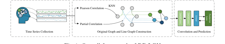 Figure 1. Overall framework of RP-LGN
Imagine a single abstract data point—a functional connection between the prefrontal cortex and the basal ganglia, derived from a \$150 fMRI scan.
First, this connection is ripped from being a mere "edge" and promoted to a full "node" in a new Line Graph. It is assigned a feature vector based on the correlation strength of the original brain regions. Next, it enters the Residual GraphSAGE assembly line. It looks at its neighboring connections, averages their information, and bundles it with its own data.
This bundled package is multiplied by the weight matrix $\theta$ to extract higher-level topological patterns, passed through the activation function $\sigma$ to clip negative values, and then added back to its original self via the residual pathway. This ensures the connection doesn't lose its original identity during processing.
After passing through multiple layers, the fully processed brain map $\phi_s$ arrives at the Bayesian classifier. Instead of multiplying by a rigid, deterministic weight to get a final answer, the classifier samples from a probability distribution. It outputs not just a diagnosis (e.g., "ADHD"), but a confidence level, factoring in the inherent noise of the raw medical data.
Optimization Dynamics
How does this architecure actually learn and converge? The model relies on Stochastic Variational Inference to navigate a notoriously difficult loss landscape.
In traditional fMRI analysis, the loss landscape is highly jagged and prone to severe overfitting because the data is high-dimensional but the sample sizes are small (small-sample bias). By introducing the Bayesian posterior (the $\Sigma$ and KL divergence terms), the loss landscape is effectively smoothed out. The model is actively penalized for being overly confident in its predictions when the data is ambiguous.
During backpropagation, gradients flow backward from the ELBO objective. The residual connections ensure that these gradients have a clear, unobstructed highway to travel all the way back to the first layer, completely bypassing the vanishing gradient problem. Iteratively, the model updates $\theta$ to extract better structural features, while simultaneously updating $\eta$ and $\Sigma$ to calibrate its uncertainty. It converges on a robust state where it can accurately distinguish between healthy and diseased brains, even when confronted with anomalous patient data.
Results, Limitations & Conclusion
Imagine the human brain as a vast, bustling country. The brain regions are the major cities, and the neural pathways between them are the highways. For years, neuroscientists and AI researchers have used Functional Magnetic Resonance Imaging (fMRI) to measure the "traffic" (blood flow) in these cities to diagnose neuropsychiatric disorders like Autism Spectrum Disorder (ASD) and Attention-Deficit/Hyperactivity Disorder (ADHD). Traditional Graph Neural Networks (GNNs) have been the go-to tool for this, treating the brain regions as nodes (cities) and the connections as edges (highways).
But here is the fundemental flaw: what if the disease doesn't destroy the city, but rather disrupts the highway? Traditional GNNs focus heavily on updating the features of the nodes, treating the connections as mere secondary attributes.
The authors of this paper recognized this blind spot and proposed a brilliant paradigm shift: the Residual-Posterior Line Graph Network (RP-LGN). They decided to make the connections the stars of the show.
The Motivation and the Mathematical Constraints
To focus on the connections, the authors used a concept from graph theory called a "line graph." In a line graph, the edges of the original graph become the nodes of the new graph.
However, they immediately hit a massive mathematical wall. If a brain atlas divides the brain into $n$ regions, a fully connected graph has $(n - 1) \times n / 2$ edges. If you convert this into a line graph, the new adjacency matrix explodes to a scale of $(n - 1)^2 \times n^2 / 4$. For a brain with hundreds of regions, you are suddenly dealing with billions of parameters. It is a computational nightmare. Furthermore, fMRI data is notoriously noisy, and medical datasets usually have small sample sizes, making massive models highly prone to overfitting.
How They Solved It: The RP-LGN Architecure
To overcome these constraints, the authors engineered a four-step pipeline:
1. Ruthless Sparsification via KNN
Before building the line graph, they had to prune the original graph. They used a K-Nearest Neighbors (KNN) approach, specifically setting $K=1$, to keep only the most critical connections based on Euclidean distance:
$$d(v_i, v_j) = \|x_i - x_j\|_2$$
To be honest, I'm not completely sure about this part either—the paper doesn't deeply justify the clinical validity of throwing away all but the first-order neighbor edges, though it undeniably solves the computational explosion.
2. The Edge-to-Node Transformation
Next, they built the line graph. The new nodes (which represent the original highways) need features. They ingeniously constructed these features by concatenating the sum of the two connected brain regions' features with the original edge weight:
$$\tilde{x}_i = \text{CONCATE}(\text{SUM}(x_i, x_j), a_{ij})$$
3. Residual GraphSAGE for Message Passing
Because line graphs lack edge weights of their own, the authors used GraphSAGE to pass messages between these new connection-nodes. To prevent "oversmoothing"—a common GNN problem where repeated message passing blurs all features into a generic mush—they added residual connections:
$$\tilde{\mathbf{X}}^{(l+1)} = \tilde{\mathbf{X}}^{(l)} + \tilde{\mathbf{Z}}^{(l)}$$
4. The Bayesian Variational Posterior
Finally, to combat the noise and small-sample overfitting, they discarded the traditional deterministic classifier. Instead, they treated the weights of the final layer as random variables with a Gaussian distribution. By using stochastic variational inference, the model doesn't just make a rigid guess; it quantifies its own uncertainty. They optimized this by maximizing the Evidence Lower Bound (ELBO):
$$S^{-1} \log p(Y|\mathbf{X}, \mathbf{A}, \theta) \geq \mathcal{L}_{VB}(\theta, \eta, \Sigma) - S^{-1}\text{KL}(q(W, \Sigma|\eta) \parallel p(W, \Sigma))$$
The Experimental Architecture and the "Victims"
The authors didn't just claim their math worked; they architected a ruthless gauntlet to prove it. They tested RP-LGN on the ABIDE I (Autism) and ADHD-200 datasets using rigorous 5-fold cross-validation.
The "victims" left in their wake were a who's-who of standard and state-of-the-art models: single classifiers like KAN, standard GNNs (GAT, GIN, GraphSAGE), and specialized brain networks like BrainNetCNN, BrainGNN, BrainGB, FBNETGEN, and BrainNetworkTransformer. RP-LGN outperformed them all.
But the definitive, undeniable evidence wasn't just a higher accuracy percentage. It came in two forms:
1. The Ablation Study: They systematically stripped away the residual connections and the Bayesian posterior. When applied to base models like SAGE, GIN, and GAT, the performance noticeably dropped, proving that these specific mechanisms were the exact reasons for the model's superiority.
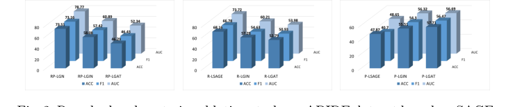 Figure 2. Resudual and posterior ablation study on ABIDE dataset based on SAGE, GIN and GAT. R: residual, P: posterior, L: line graph
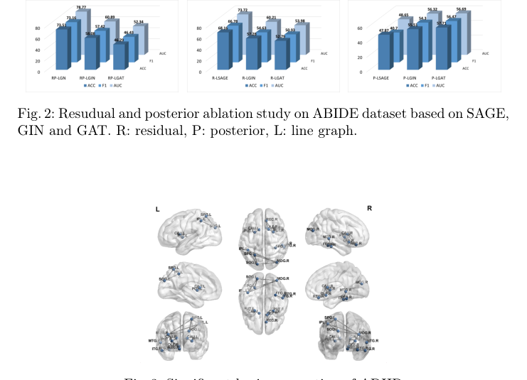 Figure 2. illustrates the average accuracy with standard error on the ABIDE dataset under different module ablations. It can be observed that the combi- nation of GraphSAGE and residual connections preserves more of the original graph information without excessively smoothing the graph, thereby maintain- ing performance. In contrast, the attention mechanism inherent in GAT and the residual posterior pattern may not integrate well, resulting in a counter- productive effect. In line graph-based models, Grad-CAM can directly analyze the importance of each connection in ADHD disease classification through node gradients. The specific connectivity visualization image is shown in Fig. 3. In this experiment, the RP-LGN model identified connections between Superior Parietal Lobule and Inferior Parietal Lobule in the prefrontal cortex, Caudate Nucleus and Putamen in the basal ganglia, Inferior Temporal Gyrus and Middle Temporal Gyrus in the temporal lobe, and the Fusiform Gyrus. The prefrontal cortex is involved in processing spatial attention and sensory information integra- tion [17]. ADHD patients often exhibit developmental delays and coordination issues in this region. In task execution, reward processing, and impulse control,
- Clinical Validation via Grad-CAM: They used gradient-based localization to visually map which "highways" the model relied on to diagnose ADHD. The model independently highlighted connections between the Superior Parietal Lobule, Caudate Nucleus, and Fusiform Gyrus. This is the smoking gun: these are the exact brain regions clinical psychiatrists have long associated with spatial attention, reward processing, and impulse control—the core deficits in ADHD. The math perfectly rediscovered the biology.
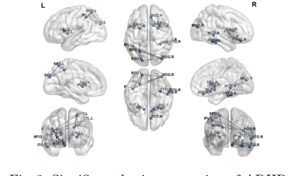 Figure 3. Significant brain connection of ADHD
Discussion Topics for Future Evolution
Based on this brilliant foundation, here are a few diverse perspectives on how we can push this represntation of brain connectivity even further:
- The $K=1$ Dilemma in Sparsification: The authors used $K=1$ to save computational overhead, but the brain is a highly integrated, multi-pathway system. Could we explore dynamic sparsification techniques, such as attention-based pruning, that keep clinically relevant long-distance connections rather than strictly relying on Euclidean nearest neighbors?
- Temporal Dynamics vs. Static Snapshots: RP-LGN treats fMRI data as a static graph of partial correlations. However, brain connectivity is highly dynamic; highways open and close depending on cognitive load. How could we integrate sliding-window temporal dynamics into a line-graph framework without triggering another parameter explosion?
- Interpreting Bayesian Uncertainty in the Clinic: The Bayesian posterior provides a mathematical quantification of uncertainty. How can we translate this mathematical variance into an actionable metric for a doctor? For instance, if the model outputs a diagnosis with high variance, could that trigger a specific secondary screening protocol in a real-world clinical setting?