PhoCoLens: Photorealistic and Consistent Reconstruction in Lensless Imaging
ISOM keeps this NeurIPS paper in the public review set because it gives readers a concrete case around PhoCoLens: Photorealistic and Consistent Reconstruction in Lensless Imaging through its mechanism, assumptions,...
Background & Academic Lineage
The Origin & Academic Lineage
The problem of lensless imaging reconstruction precisely emerged from the desire to create ultra-compact, lightweight, and cost-effective cameras. Traditional lens-based systems are bulky and expensive, limiting their application in fields requiring miniaturization, such as medical endoscopy or wearable technologies. The historical context shows that researchers began replacing conventional lenses with amplitude or phase masks placed close to the sensor to modulate incoming light, significantly reducing camera size and weight. This innovation, while promising, introduced a new challenge: without a focusing lens, the raw sensor measurements are typically blurry and unrecognizable. The camera doesn't directly record the scene but encodes it into a complex diffraction pattern, which necessitates sophisticated computational algorithms to recover a high-quality image of the original scene.
The fundamental limitation or "pain point" of previous approaches that forced the authors to write this paper stems from two main issues: achieving both photorealism and consistency in the reconstructed images, and accurately modeling the imaging process. Current algorithms often struggle with inaccurate forward imaging models and insufficient prior knowledge to reconstruct high-quality images. Specifically:
- Poor Visual Quality and Missing Details: Traditional methods, like WienerDeconv, can reconstruct images that are consistent with the ground truth but suffer from significantly degraded visual quality, often lacking rich details. Learning-based approaches, such as FlatNet-gen, attempt to enhance visual quality but frequently fail to recover high-frequency details.
- Lack of Consistency with Generative Priors: While generative restoration algorithms (e.g., DiffBIR) can inject rich details and improve photorealism, they often do so at the cost of consistency. These methods may alter image content or insert non-existent objects, leading to reconstructions that deviate from the original scene (e.g., a bird's beak with the wrong shape or fake-looking leaves).
- Inaccurate Imaging Model (Spatially Varying PSF): Most existing reconstruction algorithms simplify the lensless imaging process by assuming a shift-invariant Point Spread Function (PSF). However, in practice, the PSF is spatially varying, especially at the periphery of the field of view (FoV) where the angle of incidence increases. This mismatch between the assumed and actual imaging model leads to inaccuracies and a noticeable drop in reconstructed similarity to the original scene, particularly in peripheral areas. This occurs because the Fresnel approximation, which simplifies the light propagation model to a shift-invariant convolution, breaks down when the distance between the lensless mask and the sensor is very small (e.g., 2mm in typical lensless cameras), which is often the case. This critcal limitation means a single deconvolution kernel cannot accurately reverse the blurring across the entire image.
Intuitive Domain Terms
- Lensless Imaging: Imagine trying to take a picture with a camera that has no traditional glass lens, just a tiny, patterned window (a "mask") in front of the sensor. The light gets scrambled in a unique way as it passes through this window. Lensless imaging is all about using clever computer programs to "unscramble" that light and reconstruct a clear picture, even though no lens was used to focus it.
- Point Spread Function (PSF): Think of a single, tiny dot of light in a scene. When this dot of light passes through the lensless camera's mask and hits the sensor, it doesn't stay a perfect dot; it spreads out into a specific, often blurry, pattern. The PSF is like the unique "fingerprint" of how a single point of light gets blurred or encoded by the camera system. It tells you exactly how each point of light "spreads" onto the sensor.
- Spatially Varying Deconvolution: If the "blurring fingerprint" (PSF) changes depending on where the light comes from in the scene (e.g., light from the center of the scene blurs differently than light from the edges), a simple "un-blurring" tool won't work perfectly everywhere. Spatially varying deconvolution is like having a smart "un-blurring" process that automatically adjusts its technique for different parts of the image, applying the correct "un-blurring" method for each specific region to get a clearer, more accurate picture across the entire view.
- Range-Null Space Decomposition: Picture a very blurry photograph. This mathematical trick helps us to seperate the blurry photo into two parts. The "range space" part contains all the basic, low-detail information (like the general shapes and colors) that the camera could reliably capture, even if it's blurry. The "null space" part represents all the fine details and textures that were completely lost in the blur and cannot be directly recovered from the blurry measurement. The challenge is to reconstruct the first part accurately and then intelligently "fill in" the second part with realistic details without making things up.
- Generative Prior (from Diffusion Models): Imagine an artist who is incredibly skilled at creating realistic images from just a rough sketch. A "generative prior" from a diffusion model is like that artist. Given the basic, low-detail information (the range space content), it can "imagine" and add back the missing high-frequency, photorealistic details (the null space content) in a way that looks natural and consistent with how real-world images usually look, making the final image much more visually appealing.
Notation Table
| Notation | Description |
|---|---|
| $\hat{y}$ | Raw, multiplexed measurement captured by a lensless camera. |
| $x$ | Original scene image that the algorithm aims to reconstruct. |
| $A$ | Transfer matrix of the lensless imaging system, representing the forward imaging model. |
| $n$ | Sensor noise. |
| $A^\dagger$ | Pseudo-inverse of the transfer matrix $A$. |
| $A^\dagger A x$ | Range space component of the image $x$, representing information directly recoverable from measurements (low-frequency content). |
| $(I - A^\dagger A)x$ | Null space component of the image $x$, representing information lost during imaging (high-frequency details). |
| $I$ | Identity matrix. |
| $h$ | Point Spread Function (PSF) of the lensless system. |
| $*$ | Convolution operator. |
| $p^{(i)}$ | $i$-th learnable Point Spread Function (PSF) kernel in the SVDeconv network. |
| $\mathcal{F}$ | Discrete Fourier Transform (DFT). |
| $\mathcal{F}^{-1}$ | Inverse Discrete Fourier Transform (IDFT). |
| $\odot$ | Hadamard product (element-wise multiplication). |
| $x^{(i)}_e$ | $i$-th intermediate deconvolved image from the multi-kernel deconvolution. |
| $X_{int}$ | Spatially interpolated image from the intermediate deconvolved images. |
| $w_i(u, v)$ | Weight for the $i$-th deconvolved image at pixel $(u, v)$, based on inverse Euclidean distance. |
| $\mathbf{c}$ | Range space content, the output of the first SVDeconv stage, used as a condition for the diffusion model. |
| $\mathbf{x}_t$ | Noisy image at timestep $t$ in the diffusion process. |
| $\mathbf{\epsilon}$ | True noise vector sampled from a standard normal distribution. |
| $\mathbf{\epsilon}_\theta(\mathbf{x}_t, t, \mathbf{c})$ | Noise prediction network (parameterized by $\theta$) of the conditional diffusion model. |
| $\theta$ | Learnable parameters of the noise prediction network. |
| $\mathcal{L}_{null}$ | Loss function for the null space recovery stage, enforcing consistency in the measurement space. |
| $\mathbb{E}$ | Expectation operator. |
| $t$ | Timestep in the diffusion process. |
| $\mathcal{N}(0,1)$ | Standard normal distribution. |
| $\| \cdot \|^2$ | Squared L2 norm. |
| $\mathcal{L}_{MSE}$ | Mean Squared Error loss. |
| $\mathcal{L}_{LPIPS}$ | Learned Perceptual Image Patch Similarity loss. |
Problem Definition & Constraints
Core Problem Formulation & The Dilemma
The fundamental problem addressed by this paper is the reconstruction of photorealistic and consistent images from lensless camera measurements.
Input/Current State:
The starting point is a raw, multiplexed measurement $\hat{y} \in \mathbb{R}^{N^2}$ captured by a lensless camera. This measurement is typically blurry, unrecognizable, and lacks high-frequency details. Mathematically, the lensless imaging process can be formulated as a linear transformation of the original scene $x \in \mathbb{R}^{M^2}$ with added sensor noise $n$:
$$ \hat{y} = Ax + n $$
Here, $A \in \mathbb{R}^{N^2 \times M^2}$ is the transfer matrix of the lensless imaging system, which encodes how light from each point in the scene contributes to each sensor pixel. Previous methods often simplify this complex process as a convolution with a single, shift-invariant Point Spread Function (PSF), i.e., $y = h * x$.
Desired Endpoint (Output/Goal State):
The desired endpoint is a reconstructed image $x$ that is both photorealistic and consistent with the original scene.
* Photorealism implies a high-quality image with rich, natural-looking details, effectively recovering the high-frequency content lost during the lensless capture.
* Consistency means the reconstructed image's content must align accurately with the original scene, satisfying the condition $Ax = y$ (where $y$ is the noise-free measurement).
Missing Link or Mathematical Gap:
The exact missing link is the ability to accurately model the complex, spatially varying nature of the lensless imaging process (represented by $A$) and to effectively recover both the low-frequency (consistency-critical) and high-frequency (photorealism-critical) components of the scene from the degraded measurement. The paper leverages the range-null space decomposition to bridge this gap. Any scene $x$ can be decomposed into two orthogonal components:
$$ x = A^\dagger Ax + (I - A^\dagger A)x $$
where $A^\dagger Ax$ is the range space component (low-frequency content directly recoverable from measurements, ensuring consistency) and $(I - A^\dagger A)x$ is the null space component (high-frequency details lost in the imaging process, crucial for photorealism). The paper aims to accurately reconstruct the range space content first, and then enrich it with null space content using generative priors, all while maintaining consistency.
The Dilemma (Painful Trade-off):
The core dilemma that has trapped previous researchers is the painful trade-off between achieving high visual quality (photorealism) and maintaining data consistency (fidelity to the original scene).
* Traditional reconstruction algorithms (e.g., WienerDeconv) prioritize data consistency, producing images that align with the ground truth but are often blurry and significantly degraded in visual quality, lacking fine details. They fail to recover high-frequency information.
* Generative restoration algorithms (e.g., those using diffusion models like DiffBIR) can inject rich, photorealistic details and significantly enhance visual quality. However, they frequently "alter image content or insert non-existent objects," thereby breaking consistency with the actual scene. For instance, they might generate incorrect shapes or fake textures, as shown in Figure 1d.
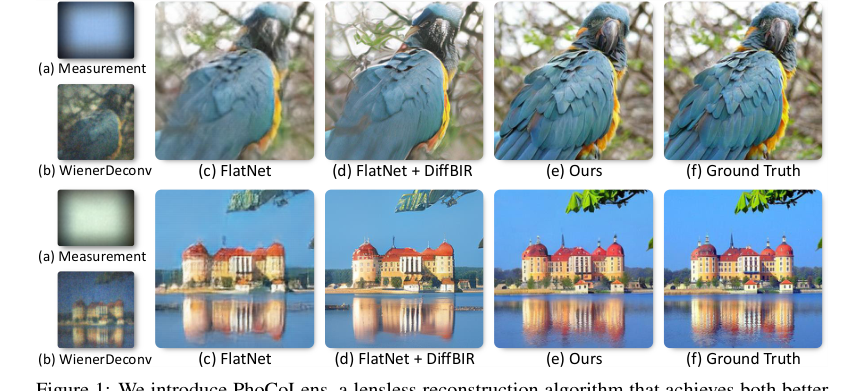 Figure 1. We introduce PhoCoLens, a lensless reconstruction algorithm that achieves both better visual quality and consistency to the ground truth than existing methods. Our method recovers more details compared to traditional reconstruction algorithms (b) and (c), and also maintains better fidelity to the ground truth compared to the generative approach (d)
This dilemma means that improving one aspect (e.g., photorealism) typically compromises the other (consistency), making it incredibly difficult to achieve both simultaneously with existing methods.
Constraints & Failure Modes
The problem of photorealistic and consistent lensless image reconstruction is insanely difficult due to several harsh, realistic constraints and common failure modes of prior approaches:
- Spatially Varying Point Spread Function (PSF):
- Physical Constraint: Unlike traditional lens-based cameras, lensless systems do not have a fixed, shift-invariant PSF across the entire field of view (FoV). The PSF varies significantly with the angle of incident light, especially at the periphery.
- Computational Constraint: Most existing reconstruction algorithms simplify the imaging process by assuming a shift-invariant PSF, which is inaccurate. Modeling the true spatially varying PSF is computationally intensive, as the full transfer matrix $A$ is "too large to compute" directly for real-world systems. This simplification leads to noticeable degradation and artifacts in reconstructed images, particularly at the boundaries, as shown in Figure 4d.
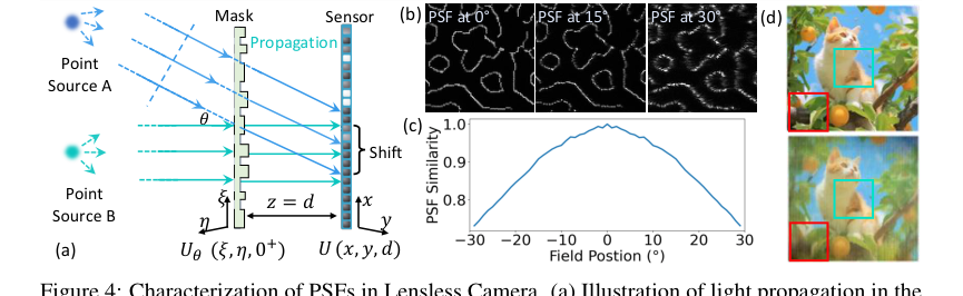 Figure 4. Characterization of PSFs in Lensless Camera. (a) Illustration of light propagation in the lensless camera: two point sources A and B at infinity emitting parallel light beams. Source A emits at angle θ relative to the optical axis, causing a PSF shift on the sensor plane This PSF shift depends on both the incident angle θ and the distance d between the sensor and the mask. (b) Simulated PSFs for light sources at angles of 0°, 15°, and 30°. (c) Inner product similarity between the on-axis PSF and off-axis PSFs at different field positions. (d) Reconstruction using PSF at 0°, degradation is more significant at the periphery (red box) than the center (green box)
-
Loss of High-Frequency Information:
- Physical Constraint: The lensless encoding process, where light is modulated by a mask, acts like a low-pass filter. This inherently causes a significant loss of high-frequency details from the scene, making the raw measurements blurry and ambiguous.
- Data-driven Constraint: Recovering these lost high-frequency details (the "null space" content) requires strong priors. Without sufficient and accurate priors, algorithms struggle to reconstruct photorealistic images, often resulting in visually degraded outputs or, if generative models are used naively, hallucinating non-existent details that break fidelity.
-
Computational Complexity of Spatially-Varying Deconvolution:
- Computational Constraint: While spatially-varying deconvolution is necessary for accurate reconstruction, previous methods in this area are "often slow, computationally intensive, and result in poor image quality, especially in complex systems."
- Calibration Burden: Many multi-kernel deconvolution approaches require "tedious multi-location PSF calibrations," which is a time-consuming and labor-intensive process, making them impractical for widespread use. The paper aims to overcome this by learning variations automatically from a single initial PSF.
-
Maintaining Data Fidelity with Generative Priors:
- Logical Constraint: Generative models, while powerful for hallucinating details, inherently operate by creating new information. A major failure mode is that they tend to "alter image content or insert non-existent objects," thereby violating the fundamental consistency requirement that the reconstructed image must align with the actual physical measurements. The challenge is to guide these generative models to produce realistic details that are consistent with the underlying data.
-
Real-time Latency (Future Limitation):
- Computational Constraint: Although not a direct constraint overcome in this paper, the authors acknowledge that the "two-stage nature of PhoCoLens and the diffusion model's sampling time hinder its real-time applicability." This implies that for applications requiring immediate feedback, such as real-time video or clinical imaging, the current computational overhead of the proposed method presents a significant hurdle.
Why This Approach
The Inevitability of the Choice
The authors of PhoCoLens faced a fundamental dilemma in lensless imaging: how to achieve both high visual quality (photorealism) and faithful representation of the original scene (consistency). Traditional state-of-the-art (SOTA) methods, such as standard deconvolution techniques like WienerDeconv, were found to be insufficient because they produced images with significantly degraded visual quality, lacking the rich details necessary for photorealism (Figure 1b). While learning-based approaches, exemplified by FlatNet-gen, improved visual quality, they still struggled to recover crucial high-frequency details, resulting in less sharp and less realistic images (Figure 1c).
The critical realization that traditional methods were insufficient came when the authors observed that even advanced generative models, like DiffBIR, which are excellent at injecting photorealistic details, often did so at the cost of consistency. These models frequently altered image content or introduced non-existent objects, such as a wrongly shaped beak or fake-looking leaves (Figure 1d), thereby breaking the fidelity to the ground truth.
Figure 1. We introduce PhoCoLens, a lensless reconstruction algorithm that achieves both better visual quality and consistency to the ground truth than existing methods. Our method recovers more details compared to traditional reconstruction algorithms (b) and (c), and also maintains better fidelity to the ground truth compared to the generative approach (d)
This indicated that a purely generative approach, while visually appealing, was not a viable sole solution for applications where accuracy to the original scene is paramount.
Furthermore, a significant limitation identified in existing reconstruction algorithms was their simplification of the lensless imaging process. Most methods assumed a shift-invariant Point Spread Function (PSF), treating the imaging as a simple convolution. However, the authors recognized that in real-world lensless systems, PSFs are inherently spatially varying, especially at different angles of incidence (Figure 4a, 4b, 4c). This mismatch between the assumed shift-invariant PSF and the actual spatially-varying PSF led to substantial inaccuracies, particularly in the peripheral field of view, where reconstructed similarity to the original scene dropped noticeably (Figure 4d).
Figure 4. Characterization of PSFs in Lensless Camera. (a) Illustration of light propagation in the lensless camera: two point sources A and B at infinity emitting parallel light beams. Source A emits at angle θ relative to the optical axis, causing a PSF shift on the sensor plane This PSF shift depends on both the incident angle θ and the distance d between the sensor and the mask. (b) Simulated PSFs for light sources at angles of 0°, 15°, and 30°. (c) Inner product similarity between the on-axis PSF and off-axis PSFs at different field positions. (d) Reconstruction using PSF at 0°, degradation is more significant at the periphery (red box) than the center (green box)
This fundamental physical reality made traditional convolutional models inherently inadequate for accurate lensless reconstruction across the entire field of view.
Comparative Superiority
PhoCoLens achieves qualitative and quantitative superiority through its novel two-stage architecture, which structurally addresses the core challenges of lensless imaging. The key structural advantage lies in its range-null space decomposition framework. This theoretical foundation allows the method to disentangle the problem into two orthogonal components: one focused on data consistency (range space) and the other on photorealism (null space).
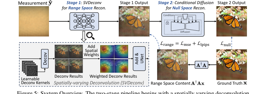 Figure 5. System Overview. The two-stage pipeline begins with a spatially varying deconvolution network mapping lensless measurements to range space. Then a conditional diffusion model for null space recovery refines details using the first stage output, achieving the final reconstruction
This is a profound advantage over previous methods that attempted to solve both simultaneously, often leading to trade-offs.
- Spatially-Varying Deconvolution (SVDeconv) for Range Space: Unlike prior methods that assume a single, shift-invariant PSF, SVDeconv learns to adapt to spatial variations in the PSF across the camera's field of view in a data-driven manner. This is a significant structural improvement, as it more accurately models the complex forward imaging process. This leads to superior reconstruction of structural integrity and low-frequency details, especially in the image periphery, where other methods fail (Figure 2, Figure 4d).
Figure 4. Characterization of PSFs in Lensless Camera. (a) Illustration of light propagation in the lensless camera: two point sources A and B at infinity emitting parallel light beams. Source A emits at angle θ relative to the optical axis, causing a PSF shift on the sensor plane This PSF shift depends on both the incident angle θ and the distance d between the sensor and the mask. (b) Simulated PSFs for light sources at angles of 0°, 15°, and 30°. (c) Inner product similarity between the on-axis PSF and off-axis PSFs at different field positions. (d) Reconstruction using PSF at 0°, degradation is more significant at the periphery (red box) than the center (green box)
Table 2 quantitatively demonstrates SVDeconv's superior performance in range space reconstruction compared to other deconvolution methods.
2. Conditional Null-Space Diffusion for Photorealism: The second stage leverages a pre-trained diffusion model, but critically, it conditions this generative process on the low-frequency content recovered from the first stage. This ensures that while high-frequency details are added for photorealism, they remain consistent with the underlying structure established by the range space reconstruction. This approach avoids the pitfalls of pure generative models (like DiffBIR) that introduce artifacts or alter content, as shown in Figure 1d.
Figure 1. We introduce PhoCoLens, a lensless reconstruction algorithm that achieves both better visual quality and consistency to the ground truth than existing methods. Our method recovers more details compared to traditional reconstruction algorithms (b) and (c), and also maintains better fidelity to the ground truth compared to the generative approach (d)
The conditioning mechanism is a structural safeguard that maintains fidelity while enhancing visual quality.
Quantitatively, PhoCoLens demonstrates overwhelming superiority. As shown in Table 1, it consistently achieves the best balance between fidelity metrics (PSNR, SSIM, LPIPS) and visual quality metrics (ManIQA, ClipIQA, MUSIQ) across both PhlatCam and DiffuserCam datasets. For instance, on PhlatCam, PhoCoLens achieves a MUSIQ score of 62.20, significantly higher than FlatNet+DiffBIR's 57.13, while also maintaining better LPIPS (0.215 vs 0.391). This indicates a method that is not just slightly better, but structurally designed to outperform previous gold standards by addressing their inherent limitations.
Alignment with Constraints
The chosen two-stage approach of PhoCoLens perfectly aligns with the dual constraints of achieving both photorealism and consistency in lensless imaging, while also addressing the underlying physical challenges.
- Addressing Spatially-Varying PSFs for Consistency: The problem's harsh requirement for accurate reconstruction across the entire field of view, despite the spatially varying nature of lensless PSFs, is directly met by the SVDeconv in the first stage. By learning and adapting to these spatial variations, SVDeconv ensures that the low-frequency content (range space) is reconstructed with high fidelity and structural integrity, laying a consistent foundation for the final image. This is a direct "marriage" between the problem's physical reality and the solution's adaptive deconvolution property.
- Leveraging Generative Priors for Photorealism while Maintaining Consistency: The constraint of achieving photorealism, which demands rich high-frequency details often lost in lensless capture, is addressed by the null-space diffusion model in the second stage. However, the critical alignment here is how this generative power is harnessed. Instead of blindly generating details, the diffusion model is conditioned on the consistent low-frequency output from the first stage. This ensures that the added high-frequency details (from the null space) enhance photorealism without violating the consistency established earlier. The mathematical framework of range-null space decomposition explicitly ensures that the null space component, when added, does not alter the measurement $y$, thus preserving consistency ($A(x - A^\dagger Ax) = 0$). This is a perfect alignment where the generative capability is constrained by the consistency requirement.
- Overcoming Insufficient Priors: The problem of insufficient priors in traditional methods, which led to degraded visual quality, is overcome by integrating a powerful pre-trained diffusion model. This model provides a strong generative prior for realistic image textures, but its application within the null-space framework ensures it's guided by the actual scene data, avoiding arbitrary hallucination.
Rejection of Alternatives
The paper explicitly and implicitly rejects several alternative approaches based on their inherent limitations in meeting the dual goals of photorealism and consistency:
- Traditional Deconvolution (e.g., WienerDeconv): These methods were rejected primarily due to their inability to produce photorealistic results. While they maintain some data consistency, their visual quality is "significantly degraded" (Section 1, Figure 1b), making them unsuitable for high-quality image reconstruction.
- Learning-Based Deconvolution (e.g., FlatNet-gen): While an improvement over traditional methods, these approaches were found to "often fail to recover high-frequency details" (Section 1, Figure 1c). This limitation meant they could not achieve the desired level of photorealism, leading to a lack of sharpness and fine textures.
- Generative Models with Direct Priors (e.g., DiffBIR): These methods, while excellent at injecting rich details and enhancing visual quality, were rejected because they "may also alter image content or insert non-existent objects, breaking consistency" (Section 1, Figure 1d). The authors provide clear examples of distorted objects (e.g., the beak shape) and fake textures, demonstrating that their photorealism comes at an unacceptable cost to fidelity.
- Methods Assuming Shift-Invariant PSFs: A major implicit rejection is of any method that simplifies the lensless imaging process by assuming a shift-invariant PSF. As detailed in Section 3.2 and illustrated in Figure 4d, this assumption leads to "inaccuracies" and a "noticeable drop in the reconstructed similarity to the original scene, especially in the peripheral field of view." PhoCoLens's SVDeconv stage was specifically designed to overcome this fundamental flaw, making any shift-invariant approach inherently inferior for real-world lensless systems.
- Zero-shot Diffusion Models (e.g., DDNM+): While mentioned as a category of inverse imaging with diffusion models, the paper's approach integrates "supervised fine-tuning with a theoretical framework based on range-null space decomposition" (Section 2). This implies a rejection of purely zero-shot methods for this specific problem, likely because they might lack the fine-grained control or consistency guarantees that supervised training within the decomposition framework provides. Table 3 shows that DDNM+ performs significantly worse than PhoCoLens in both fidelity and visual quality metrics for null space recovery.
Mathematical & Logical Mechanism
The Master Equation
The core mathematical engine driving this paper, particularly for achieving photorealism and consistency in the second stage of the reconstruction, is the optimization objective for the null space diffusion model. This equation ensures that the high-frequency details generated by the diffusion model remain consistent with the underlying physics of the lensless imaging system. It is formally expressed as:
$$ \min_\theta \mathcal{L}_{null} = \min_\theta \mathbb{E}_{\mathbf{x},t,\mathbf{c},\mathbf{\epsilon} \sim \mathcal{N}(0,1)} \left[ \left\| A(\mathbf{\epsilon}_\theta(\mathbf{x}_t, t, \mathbf{c}) - \mathbf{\epsilon}) \right\|^2 \right] $$
This equation is derived from the fundamental principle of range-null space decomposition, which posits that any image $\mathbf{x}$ can be split into a range space component $A^\dagger A \mathbf{x}$ (representing information directly observable by the camera) and a null space component $(I - A^\dagger A) \mathbf{x}$ (representing details lost in the imaging process but crucial for photorealism). The objective here is to ensure that the residual content added by the generative model, which should ideally reside in the null space, does not violate the consistency with the forward imaging model.
Term-by-Term Autopsy
Let's dissect this equation piece by piece to understand its role and significance:
- $\min_\theta$: This is the standard minimization operator, indicating that the goal is to find the optimal set of parameters $\theta$ for the neural network.
- $\theta$: These are the learnable parameters of the noise prediction network, $\mathbf{\epsilon}_\theta$. This network is a deep learning model, typically a U-Net, that learns to predict the noise component in a noisy image.
- $\mathcal{L}_{null}$: This symbol represents the loss function specifically designed for the null space recovery stage. Its minimization guides the diffusion model to generate consistent and photorealistic details.
- $\mathbb{E}_{\mathbf{x},t,\mathbf{c},\mathbf{\epsilon} \sim \mathcal{N}(0,1)}$: This denotes the expectation operator, meaning we are averaging the loss over multiple random samples.
- $\mathbf{x}$: This is the ground truth, clean image that the model aims to reconstruct. It's the ideal target.
- $t$: This represents a timestep in the forward diffusion process, indicating how much noise has been added to the image. Diffusion models operate by progressively adding noise and then learning to reverse this process.
- $\mathbf{c}$: This is the condition for the diffusion model, specifically the range space content $A^\dagger A \mathbf{x}$ reconstructed from the first stage. It provides the low-frequency, consistent information that the generative model must adhere to.
- $\mathbf{\epsilon} \sim \mathcal{N}(0,1)$: This is the actual noise vector sampled from a standard normal distribution, which is added to the clean image $\mathbf{x}$ to create the noisy image $\mathbf{x}_t$.
- $\| \cdot \|^2$: This is the squared L2 norm, a common choice for loss functions in regression tasks. It measures the squared Euclidean distance between two vectors, penalizing larger errors more significantly. The authors chose this because it's a straightforward and effective way to quantify the difference between the predicted noise and the actual noise.
- $A$: This is the transfer matrix of the lensless imaging system. It mathematically describes how a scene $\mathbf{x}$ is transformed into a measurement $\mathbf{y}$ by the camera (i.e., $\mathbf{y} = A\mathbf{x}$). Its role here is critical: it projects the noise prediction error into the measurement space.
- $\mathbf{\epsilon}_\theta(\mathbf{x}_t, t, \mathbf{c})$: This is the output of the neural network, parameterized by $\theta$. Given a noisy image $\mathbf{x}_t$, the current timestep $t$, and the range space condition $\mathbf{c}$, this network predicts the noise component $\mathbf{\epsilon}$ that was added to the original image.
- $(\mathbf{\epsilon}_\theta(\mathbf{x}_t, t, \mathbf{c}) - \mathbf{\epsilon})$: This term represents the error in the noise prediction. The network is trying to make its prediction $\mathbf{\epsilon}_\theta$ as close as possible to the true noise $\mathbf{\epsilon}$.
- $A(\mathbf{\epsilon}_\theta(\mathbf{x}_t, t, \mathbf{c}) - \mathbf{\epsilon})$: This is the most crucial part of the loss. Instead of simply minimizing the difference between predicted and actual noise, the authors apply the transfer matrix $A$ to this difference. This ensures that the effect of the noise prediction error, when projected into the measurement space, is minimized. In essence, it forces the generative model to predict noise that, if it were to be "imaged" by the lensless camera, would result in zero measurement error. This directly enforces the consistency requirement that any generated details (which come from the null space) should not alter the measurement that would be obtained from the range space content. The use of multiplication by $A$ here, rather than, say, addition, is fundamental to projecting the error into the measurement domain, aligning with the physical forward model.
Step-by-Step Flow
The PhoCoLens method operates in a clever two-stage pipeline, akin to a sophisticated assembly line, where each stage refines the image reconstruction with specific objectives.
Figure 5. System Overview. The two-stage pipeline begins with a spatially varying deconvolution network mapping lensless measurements to range space. Then a conditional diffusion model for null space recovery refines details using the first stage output, achieving the final reconstruction
Stage 1: Range Space Reconstruction with Spatially-Varying Deconvolution (SVDeconv)
- Initial Measurement Input: The process begins with a raw, blurry, and noisy lensless measurement $\hat{y}$. This is the initial abstract data point, a complex diffraction pattern captured by the sensor.
- Multi-Kernel Deconvolution: This measurement $\hat{y}$ enters the SVDeconv network. Here, it's not just one deconvolution, but many. The network maintains a set of $K \times K$ learnable Point Spread Function (PSF) kernels, $p^{(i)}$, each specialized for a different spatial region of the image.
- The measurement $\hat{y}$ and each kernel $p^{(i)}$ are first transformed into the frequency domain using the Discrete Fourier Transform ($\mathcal{F}$).
- In the frequency domain, an element-wise multiplication (Hadamard product $\odot$) is performed between the transformed measurement and each transformed kernel. This is the frequency-domain equivalent of deconvolution, effectively "undoing" the blurring caused by the lensless system for that specific region.
- Each result is then transformed back to the spatial domain using the Inverse Discrete Fourier Transform ($\mathcal{F}^{-1}$), yielding $K \times K$ intermediate deconvolved images, $x^{(i)}_e$. Each $x^{(i)}_e$ is a preliminary reconstruction, optimized for a particular field point.
- Spatially-Varying Interpolation: These $K \times K$ intermediate images are then seamlessly stitched together. For every pixel $(u, v)$ in the final output, a weighted sum of the corresponding pixels from all $x^{(i)}_e$ images is computed. The weights $w_i(u, v)$ are determined by the inverse Euclidean distance from the pixel $(u, v)$ to the center of the $i$-th PSF kernel. This means that a pixel's value is predominantly influenced by the deconvolution kernel that is spatially closest to it, creating a unified image $X_{int}$ that adapts to the spatially varying nature of the PSF.
- Refinement U-Net: The interpolated image $X_{int}$ then passes through a U-Net. This neural network acts as a final clean-up crew, removing any remaining noise and artifacts, and further refining the image to produce the range space content, $\mathbf{c}$. This $\mathbf{c}$ is a consistent, low-frequency representation of the scene, ready for the next stage.
Stage 2: Null Space Content Recovery with Conditional Diffusion
- Noisy Image Generation & Conditioning: The range space content $\mathbf{c}$ from Stage 1 is now used as a condition. Simultaneously, a ground truth image $\mathbf{x}$ is progressively corrupted by adding random noise $\mathbf{\epsilon}$ over several timesteps $t$, resulting in a noisy image $\mathbf{x}_t$.
- Conditional Noise Prediction: The noisy image $\mathbf{x}_t$, the current timestep $t$, and the range space condition $\mathbf{c}$ are fed into a conditional diffusion model's noise prediction network, $\mathbf{\epsilon}_\theta$.
- The condition $\mathbf{c}$ is not just concatenated; it's integrated deeply. A conditional encoder extracts multi-scale features from $\mathbf{c}$, which then modulate the intermediate feature maps within the $\mathbf{\epsilon}_\theta$ network's residual blocks. This ensures that the generative process is tightly guided by the consistent low-frequency information.
- The network $\mathbf{\epsilon}_\theta$ processes these inputs and outputs its best guess for the noise $\mathbf{\epsilon}$ that was originally added to create $\mathbf{x}_t$.
- Consistency Enforcement (Loss Calculation): The predicted noise $\mathbf{\epsilon}_\theta$ is compared to the actual noise $\mathbf{\epsilon}$. The crucial step is applying the transfer matrix $A$ to their difference, $A(\mathbf{\epsilon}_\theta - \mathbf{\epsilon})$. The squared L2 norm of this result forms the $\mathcal{L}_{null}$ loss. This ensures that any discrepancies between predicted and actual noise, when viewed through the lensless camera's forward model, are minimized.
- Iterative Denoising (Inference): During inference, the diffusion model starts with a purely random noise image. Over many timesteps, it iteratively uses the learned $\mathbf{\epsilon}_\theta$ network to predict and subtract noise, gradually transforming the random noise into a photorealistic image. At each step, the range space content $\mathbf{c}$ continuously guides the generation, ensuring that the added high-frequency details are consistent with the low-frequency structure, ultimately yielding the final, high-quality reconstructed image.
Optimization Dynamics
The PhoCoLens system learns and converges through a two-pronged optimization strategy, each tailored to its respective stage.
Stage 1: SVDeconv Optimization
The first stage, SVDeconv, is trained to reconstruct the range space content $A^\dagger A \mathbf{x}$. Its optimization involves learning the parameters of the multi-kernel deconvolution and the refinement U-Net.
- Loss Function: The training objective for SVDeconv is a combination of Mean Squared Error (MSE) loss and LPIPS (Learned Perceptual Image Patch Similarity) loss.
- MSE Loss: This is a pixel-wise fidelity loss, aiming to minimize the squared difference between the reconstructed range space content and the ground truth range space content. It ensures that the model accurately recovers the low-frequency information.
- LPIPS Loss: This is a perceptual loss that measures the similarity between images in a feature space learned by a pre-trained deep neural network. It's crucial for ensuring that the reconstructed images look visually pleasing and realistic to human observers, even if pixel values aren't perfectly matched.
- Gradient Behavior: Gradients from both MSE and LPIPS losses are backpropagated through the refinement U-Net and, importantly, through the differentiable multi-kernel deconvolution layer. This allows the network to learn the optimal PSF kernels $p^{(i)}$ that best adapt to spatial variations in the lensless imaging system. The gradients guide the kernels to effectively "undo" the spatially-varying blur.
- State Updates: The Adam optimizer is employed to iteratively update the learnable PSF kernels and the U-Net parameters. The learning rates are carefully chosen (e.g., 4e-9 for PhlatCam deconvolution kernels, 3e-5 for U-Net) to ensure stable and effective convergence. The model learns to automatically adapt to spatial PSF variations in a data-driven manner, eliminating the need for tedious multi-location PSF calibrations.
Stage 2: Null Space Diffusion Optimization
The second stage, the conditional diffusion model, is optimized to recover the null space content, adding photorealistic high-frequency details while maintaining consistency.
- Loss Function: The primary loss for this stage is $\mathcal{L}_{null}$, as defined by the master equation. This loss is unique because it applies the transfer matrix $A$ to the noise prediction error.
- Loss Landscape Shaping: The application of $A$ to the error term $A(\mathbf{\epsilon}_\theta - \mathbf{\epsilon})$ profoundly shapes the loss landscape. It creates a landscape where the minimum corresponds to a state where the generated high-frequency details (derived from the predicted noise) are "invisible" to the lensless camera's forward model. In other words, any details added by the diffusion model must lie in the null space of $A$, meaning they do not change the measurement $\mathbf{y}$ when projected through $A$. This prevents the generative model from hallucinating details that contradict the physical measurements, thus enforcing data consistency.
- Gradient Behavior: Gradients are computed through the entire expression, including the $A$ operator, and backpropagated through the noise prediction network $\mathbf{\epsilon}_\theta$. These gradients guide $\mathbf{\epsilon}_\theta$ to learn to predict noise such that the resulting reconstructed image, when passed through the forward imaging model $A$, remains consistent with the low-frequency range space content $\mathbf{c}$. This is a sophisticated way to ensure that the generative model's output aligns with the physical constraints of the lensless system.
- State Updates: The diffusion model is trained for a significant number of epochs (e.g., 200 epochs). The paper mentions leveraging a pre-trained diffusion model (like Stable Diffusion) with frozen weights, and primarily training supplementary conditioning modules. This strategy allows the model to harness the powerful generative capabilities of large pre-trained models while fine-tuning them to the specific task and consistency requirements of lensless imaging. The conditioning mechanism, which modulates internal feature maps based on $\mathbf{c}$, is iteratively updated to ensure that the generated high-frequency content is coherent with the low-frequency structure provided by the first stage. This iterative refinement of the conditioning ensures the final output is both photorealistic and consistent.
Results, Limitations & Conclusion
Experimental Design & Baselines
To rigorously validate PhoCoLens, the authors architected a comprehensive experimental setup, pitting their novel two-stage approach against a diverse array of "victim" baseline models across two distinct real-world lensless imaging datasets.
The experiments leveraged two popular lensless camera systems:
- PhlatCam Dataset [17]: Comprising 10,000 images across 1,000 classes, resized to 384x384 pixels, with raw captures at 1280x1480 pixels. A split of 990 classes for training and 10 for testing was used.
- DiffuserCam Dataset [27]: Consisting of 25,000 paired images (lensless measurement + ground truth) captured simultaneously. These images, originally 1080x1920 pixels, were downsampled to 270x480 and then cropped to a final resolution of 210x380 pixels. The dataset was split into 24,000 for training and 1,000 for testing.
To definitively prove their mathematical claims, the evaluation employed a dual set of metrics, assessing both consistency (fidelity) and photorealism (visual quality):
- Full-reference metrics for consistency: Peak Signal-to-Noise Ratio (PSNR), Structural Similarity Index Measure (SSIM) [42], and Learned Perceptual Image Patch Similarity (LPIPS) [51]. Lower LPIPS values indicate better fidelity.
- Non-reference metrics for photorealism: Multi-dimension Attention Network for No-Reference Image Quality Assessment (ManIQA) [45], CLIP-based Image Quality Assessment (ClipIQA) [39], and Multi-scale Image Quality Transformer (MUSIQ) [16]. Higher values for these metrics generally indicate better visual quality.
The implementation details were meticulously outlined to ensure reproducibility. The SVDeconv network utilized 3x3 PSF kernels, initialized with a single calibrated PSF, and a U-Net adapted from existing architectures (Le-ADMM-U for DiffuserCam, FlatNet-gen for PhlatCam). Training spanned 100 epochs with a batch size of 5, using the Adam optimizer [18]. Specific learning rates were set for the U-Net and deconvolution kernels, along with MSE and LPIPS loss weights (1 and 0.05, respectively). For the null-space diffusion stage, the SVDeconv output served as input conditions, and the model was trained for 200 epochs, leveraging a pre-trained Stable Diffusion [32] model with frozen weights, focusing only on training the supplementary conditioning modules.
The "victims" (baseline models) against which PhoCoLens was compared included:
- Traditional methods: WienerDeconv [44] (Tikhonov regularized reconstruction) and ADMM [7] (total variation regularization).
- Learning-based methods: Le-ADMM-U [27] (deep unrolled network), MMCN [49], UPDN [19] (unrolled primal-dual networks), and FlatNet-gen [17] (feedforward deconvolution).
- Diffusion-based methods: DDNM+ [41] (zero-shot inverse imaging with pre-trained Stable Diffusion) and FlatNet+DiffBIR [23] (FlatNet-gen outputs enhanced by a pre-trained blind image restoration diffusion model).
Furthermore, the authors conducted targeted ablation studies to ruthlessly prove the contribution of each core component:
- Spatially-varying Deconvolution (SVDeconv): Compared against Le-ADMM-U, SingleDeconv (using a single kernel), and MultiWienerNet [48] for both range space and original content reconstruction.
- Null-space Diffusion: Compared against conditional diffusion models like DiffBIR [23] and StableSR [39], and the zero-shot inverse imaging method DDNM+ [41].
- Range Content Conditions: An ablation where the first-stage reconstructed range content was replaced with outputs from WienerDeconv, FlatNet-gen, and SVD-OC (SVDeconv trained with original content) to condition the second-stage diffusion.
What the Evidence Proves
The evidence presented in the paper provides definitive, undeniable proof that PhoCoLens achieves a superior balance of photorealism and consistency in lensless imaging reconstruction, outperforming all baselines.
Overall Superiority:
Table 1 unequivocally demonstrates PhoCoLens's dominance. Across both the PhlatCam and DiffuserCam datasets, our method consistently achieves the best performance in nearly all full-reference metrics (PSNR, SSIM, LPIPS↓) for consistency and non-reference metrics (ManIQA, ClipIQA, MUSIQ) for visual quality. For instance, on PhlatCam, PhoCoLens achieves a PSNR of 22.07, SSIM of 0.601, and LPIPS of 0.215, significantly surpassing the next best methods like FlatNet-gen (PSNR 20.53, SSIM 0.549, LPIPS 0.375) and FlatNet+DiffBIR (PSNR 19.96, SSIM 0.544, LPIPS 0.391). This quantitative evidence is further reinforced by the qualitative comparisons in Figures 1, 6, and 7, where PhoCoLens's reconstructions are visually closest to the ground truth, exhibiting both sharp details and accurate content.
Figure 1. We introduce PhoCoLens, a lensless reconstruction algorithm that achieves both better visual quality and consistency to the ground truth than existing methods. Our method recovers more details compared to traditional reconstruction algorithms (b) and (c), and also maintains better fidelity to the ground truth compared to the generative approach (d)
Efficasy of Spatially-varying Deconvolution (SVDeconv):
The paper's core claim regarding the importance of spatially-varying deconvolution is ruthlessly proven by Table 2 and Figures 2, 8, and A3. Table 2 shows that SVDeconv (Ours) consistently outperforms other deconvolution methods (Le-ADMM-U, SingleDeconv, MultiWienerNet) in reconstructing both range space content and original content. For example, on PhlatCam, SVDeconv achieves a range space PSNR of 26.97, significantly higher than SingleDeconv's 25.61. This is crucial because traditional methods, like SingleDeconv, assume a shift-invariant PSF, which is inaccurate in real-world lensless systems. Figures 2 and 8 visually highlight this, showing that SVDeconv (right) reconstructs fine details, especially at the periphery, with far greater accuracy than methods using a single kernel (left). The red boxes in Figure 4d and the white dashed boxes in Figure 8 clearly illustrate how our SVDeconv mechanism effectively mitigates artifacts and preserves details in peripheral regions, where PSF variations are most pronounced.
Figure 4. Characterization of PSFs in Lensless Camera. (a) Illustration of light propagation in the lensless camera: two point sources A and B at infinity emitting parallel light beams. Source A emits at angle θ relative to the optical axis, causing a PSF shift on the sensor plane This PSF shift depends on both the incident angle θ and the distance d between the sensor and the mask. (b) Simulated PSFs for light sources at angles of 0°, 15°, and 30°. (c) Inner product similarity between the on-axis PSF and off-axis PSFs at different field positions. (d) Reconstruction using PSF at 0°, degradation is more significant at the periphery (red box) than the center (green box)
Figure A3 further solidifies this by showing that SVDeconv's outputs maintain high visual consistency with the ground truth's low-frequency structure, unlike FlatNet, which introduces incorrect high-frequency details.
Definitive Evidence for Null-space Diffusion:
The effectiveness of our null-space diffusion for photorealism while maintaining consistency is undeniably demonstrated in Table 3 and Figure 9. Our method achieves the highest PSNR (22.07), SSIM (0.601), and lowest LPIPS (0.215) on PhlatCam for null space recovery, significantly outperforming other diffusion-based approaches like DiffBIR (PSNR 16.21, SSIM 0.432, LPIPS 0.502) and StableSR (PSNR 14.93, SSIM 0.446, LPIPS 0.624). Qualitatively, Figure 9 shows that our method produces images that are both visually appealing and faithful to the original scene, whereas competitors like DiffBIR can introduce artifacts or distort content (e.g., the "wrong shape" beak in Figure 1d, or the human hand transferred into clothes in Figure 7). This proves that conditioning the diffusion model on the low-frequency content from the first stage effectively guides it to reconstruct realistic high-frequency details without sacrificing fidelity.
Impact of Range Content Conditions:
The ablation study on range content conditions, summarized in Table 4 and Figure 10, provides compelling evidence for the importance of using our first-stage output as a condition. When our reconstructed range content is used to condition the diffusion model, it consistently leads to better reconstruction consistency (higher PSNR, SSIM, lower LPIPS) compared to using outputs from baselines like WienerDeconv or FlatNet-gen. This is because these alternative conditions introduce artifacts that hinder the second stage's ability to recover the original image accurately. The visual improvements in Figure 10 further underscore that our two-stage pipeline, with its carefully chosen conditioning, is critical for achieving the observed superior performance.
Limitations & Future Directions
While PhoCoLens marks a significant advancement in lensless imaging, it's important to acknowledge its current limitations and consider avenues for future development.
One primary limitation of our approach is its real-time applicability. The two-stage architecture, particularly the diffusion model's sampling process in the second stage, introduces a computational overhead that currently hinders its use in real-time photo and video capture scenarios. This is a common challenge with high-quality generative models, and addressing it would unlock a much broader range of applications for lensless cameras.
Additionally, despite achieving superior fidelity, the diffusion model, by its generative nature, may still introduce high-frequency details that deviate slightly from the original scene, especially in areas that are inherently smooth or lack intricate textures. While this is a trade-off for enhanced photorealism, it suggests there's still room to refine the balance between generative creativity and strict data fidelity.
Looking ahead, several exciting directions can further evolve these findings:
- Accelerating Diffusion Model Sampling: A crucial future direction is to research and implement techniques to significantly speed up the diffusion model's sampling process. This could involve exploring faster sampling algorithms, distillation techniques, or hardware-aware optimizations. Achieving real-time performance would transform lensless cameras into viable solutions for dynamic scenes, enabling applications in areas like autonomous navigation, surveillance, and interactive imaging.
- Exploring 3D Spatially Varying PSF Effects: The current work primarily focuses on 2D image reconstruction. However, lensless cameras inherently capture 3D scene information encoded within their complex diffraction patterns. Future work could delve into modeling and leveraging 3D spatially varying Point Spread Functions (PSFs) to reconstruct not just 2D photorealistic images but also depth maps or full 3D scene representations. This would open doors to novel 3D imaging applications with ultra-compact devices, such as volumetric microscopy or augmented reality.
- Adaptive Consistency-Photorealism Trade-off: The current method strikes a fixed balance between consistency and photorealism. Future research could explore dynamic or user-controlled mechanisms to adjust this trade-off. For instance, in medical imaging, strict consistency might be paramount, while for artistic applications, greater photorealism (even with slight deviations) might be preferred. Developing a framework that allows for adaptive weighting of fidelity and generative priors could cater to a wider range of user needs and application domains.
- Robustness to Diverse Imaging Conditions: While tested on two popular lensless systems, the performance under extreme or novel imaging conditions (e.g., very low light, highly dynamic scenes, different mask designs) could be further investigated. Enhancing the model's robustness and generalization capabilities to a broader spectrum of lensless camera designs and environmental factors would be a valuable contribution.
- Ethical Considerations and Privacy-Preserving Designs: As highlighted in the broader impacts section, the proliferation of small, discreet lensless cameras raises significant privacy concerns. Future research should not only focus on technical improvements but also on integrating privacy-preserving mechanisms directly into the imaging and reconstruction pipeline. This could involve exploring on-device processing to minimize data transmission, differential privacy techniques, or designing lensless systems that inherently limit the scope of captured information to protect individual privacy rights. This cross-disciplinary effort, involving engineers, ethicists, and policymakers, is essential to ensure responsible technological advancement.
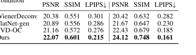 Table 2. Comparison of deconvolution methods for range space reconstruction and original content reconstruction
 Table 4. Comparison of different diffusion conditions