On the Power of Small-size Graph Neural Networks for Linear Programming
Graph neural networks (GNNs) have recently emerged as powerful tools for addressing complex optimization problems.
Background & Academic Lineage
The Origin & Academic Lineage
The problem addressed in this paper originates from the burgeoning field of Learning to Optimize (L2O), which seeks to enhance the efficency of traditional optimization processes by integrating machine learning techniques. Within L2O, Graph Neural Networks (GNNs) have recently gained significant traction for their ability to tackle complex optimization problems, particularly Linear Programming (LP) and Mixed Integer Linear Programming (MILP).
Historically, GNNs have been theoretically shown to universally approximate the solution mapping functions for LPs. However, these foundational theorectical results, notably from Chen et al. [8] and Qian et al. [29], typically postulate that GNNs require a substantial number of parameters or polynomial depth relative to the problem dimension to achieve arbitrary precision. This theoretical requirement stems from their reliance on concepts like the universal approximation theorem for multi-layer perceptrons (MLPs).
The fundamental limitation, or "pain point," of these previous approaches is the stark discrepency between theoretical predictions and empirical observations. In practice, researchers have found that relatively small GNNs—often with modest width and fewer than ten layers—can effectively solve LPs with hundreds of nodes and constraints, achieving good performance despite their limited size. This practical success, juxtaposed with the theoretical demand for large, complex GNNs, created a significant gap. The authors wrote this paper precisely to bridge this gap, seeking to provide a theoretical foundation for why and when small-size GNNs can effectively solve LPs, particularly packing and covering LPs.
Intuitive Domain Terms
- Linear Programming (LP): Imagine you have a recipe for baking cookies, but you only have a limited amount of flour, sugar, and butter. You want to bake as many cookies as possible (or maximize your profit if you sell them) while staying within your ingredient limits. Linear programming is a mathematical tool that helps you figure out the best combination of cookies to bake to achieve your goal, given these simple, straight-line constraints.
- Graph Neural Networks (GNNs): Think of a social network where people are nodes and friendships are connections. A GNN is like a smart detective who learns about each person by talking to them and their friends, then uses that collective information to understand the entire network. In optimization, it learns from the relationships between variables and constraints in a problem.
- Packing LPs: Picture trying to fit as many different-sized boxes as possible into a truck without exceeding its weight or volume capacity. A packing LP is an optimization problem that helps you find the best way to "pack" things (like resources or items) into a limited space or budget, ensuring you don't go over any limits.
- Covering LPs: Imagine you need to place security cameras to cover all entrances of a building, and each camera covers a few specific entrances. A covering LP helps you find the minimum number of cameras needed to "cover" all the entrances, ensuring every entrance is monitored.
- Polylogarithmic-depth, Constant-width GNNs: This describes a GNN that's "shallow" (polylogarithmic depth means its layers grow very slowly with problem size, like $\log(\text{size})$ or $\log^2(\text{size})$) and "skinny" (constant width means each layer has a fixed, small number of internal processing units, regardless of how big the problem gets). It's like a very efficient, compact computational machine that can still solve big problems.
Notation Table
| Notation | Description |
|---|---|
| $A$ | Constraint matrix of the LP ($n \times m$) |
| $x$ | Primal variable vector ($m \times 1$) |
| $y$ | Dual variable vector ($n \times 1$) |
| $X^k$ | Primal variable matrix at iteration $k$ ($m \times d$) |
| $Y^k$ | Dual variable matrix at iteration $k$ ($n \times d$) |
| $d$ | Channel dimension for expanded variables |
| $n$ | Number of constraints (rows in $A$) |
| $m$ | Number of primal variables (columns in $A$) |
| $K$ | Total number of GNN layers (iterations) |
| $\mu$ | Scaling parameter for ELU input |
| $\epsilon$ | Approximation precision parameter |
| $\text{ELU}(\cdot)$ | Exponential Linear Unit activation function |
| $\text{ReLU}(\cdot)$ | Rectified Linear Unit activation function |
| $f_{\theta^k}(\cdot)$ | Learnable function for primal variable update (multiplicative) |
| $g_{\theta^k}(\cdot)$ | Learnable function for primal variable update (additive) |
| $W^k$ | Learnable weight matrix for channel mixing ($d \times d$) |
| $\odot$ | Hadamard product (element-wise multiplication) |
| $1_{p \times q}$ | All-ones matrix of dimension $p \times q$ |
| $\Theta$ | Set of all learnable parameters in GD-Net |
| $obj_i$ | Predicted objective value for instance $i$ |
| $obj^*_i$ | Optimal objective value for instance $i$ |
| R. Gap | Relative Gap: $|obj_i - obj^*_i| / obj^*_i$ |
| A. Gap | Absolute Gap: $|obj_i - obj^*_i|$ |
Problem Definition & Constraints
Core Problem Formulation & The Dilemma
The paper addresses a significant gap between theoretical understanding and practical observations regarding Graph Neural Networks (GNNs) for Linear Programming (LP) problems.
Input/Current State:
The starting point is the established theoretical result that GNNs can universally approximate the solution mapping functions of LP problems. However, these theoretical proofs typically necessitate GNNs with a large number of parameters or a depth polynomial in the problem dimension. Concurrently, empirical evidence consistently demonstrates that relatively small GNNs (e.g., with modest width and fewer than ten layers) can effectively solve LPs, achieving good performance in practice.
Desired Endpoint/Goal State:
The primary goal is to provide a robust theoretical foundation that explains why and when small-size GNNs are effective for solving LPs. Specifically, the paper aims to prove that GNNs with polylogarithmic depth and constant width are sufficient to approximate the solution mapping for a broad class of LPs, namely packing and covering LPs, with arbitrary precision. This theoretical validation for smaller, more efficient GNNs would then guide the development of parameter-efficient models for Learning to Optimize (L2O) and potentially accelerate traditional LP and Mixed Integer Linear Programming (MILP) solvers.
Missing Link/Mathematical Gap:
The exact missing link is the theoretical justification for the empirical success of small-sized GNNs. Previous theoretical work on GNNs' universal approximation capabilities for LPs relied on assumptions of large model sizes (e.g., large parameter counts or polynomial depth), creating a disconnect with observed practical efficiency. This paper attempts to bridge this gap by mathematically demonstrating that GNNs can simulate a variant of gradient descent algorithms on carefully selected potential functions, thereby achieving strong approximation guarantees with significantly smaller architectures (polylogarithmic depth and constant width).
Painful Trade-off & The Dilemma:
The core dilemma is the "significant discrepancy between theoretical predictions and practical observations" (Abstract, p.1). Researchers have been "trapped" by a trade-off where achieving strong theoretical guarantees for GNNs in LP solving traditionally required large, computationally intensive models, while practical implementations often found smaller, more efficient models to be surprisingly effective. This creates a painful choice between theoretical rigor (demanding large models with high computational costs and extensive training data) and practical efficiency (achieved by smaller models whose success lacked formal explanation). The paper explicitly frames this as an "intriguing open question: When and why can small-size GNNs effectively solve LPs?" (Introduction, p.2), highlighting the need to reconcile this theoretical-empirical divide.
Constraints & Failure Modes
The problem of developing efficient and theoretically grounded GNNs for LP solving is constrained by several harsh, realistic walls:
- Computational Resource Limits: Larger GNNs inherently demand "more training examples and higher computational resources" (Introduction, p.2). This is a practical constraint that limits the scalability and applicability of GNNs if theoretical guarantees always require massive models. The drive for "parameter-efficient models" (Introduction, p.2) directly addresses this.
- Problem Complexity and Scale: LPs, particularly packing and covering LPs, can involve hundreds of nodes and constraints (Introduction, p.2). Solving these large-scale problems efficiently within acceptable timeframes is a significant challenge.
- Theoretical Bounds on Model Size: Prior theoretical results for general LPs required GNNs to have "large parameter sizes" or "depth... polynomial in the problem dimension" (Introduction, p.2). This theoretical barrier made it difficult to prove the effectiveness of smaller GNNs, despite their empirical success.
- Approximation Precision Requirements: The goal is to achieve a $(1+\epsilon)$-approximate solution (Section 1.1, p.2). This means the GNN must not only be efficient but also maintain a high level of solution quality, which is a non-trivial task when reducing model size.
- Solution Feasibility: A common failure mode for machine learning-based optimization solvers is producing infeasible solutions. The
x_finalory_finaloutput by the GD-Net might not satisfy all LP constraints (e.g., $x \ge 0$, $Ax \le 1$). The paper addresses this with a "Feasibility resortation" post-processing procedure (p.7, p.8), indicating this as a critical constraint to overcome. - Non-Differentiable Operations: The underlying gradient descent algorithms (Algorithms 1 and 2) involve conditional updates (if-else statements) and
maxoperations, which are non-differentiable. Directly translating these into neural networks is problematic. The authors circumvent this by approximating Heaviside step functions with learnable sigmoid functions (Equations 4, 5, 6, p.6) and using ReLU for non-negativity, effectively transforming non-differentiable logic into a differentiable neural network architecture. This is a key technical constraint in unrolling iterative algorithms. - Hardware Memory Limitations: While not explicitly stated as a hard limit hit, the experimental setup mentions "2.95 TB RAM" (Section E, p.16), implying that memory can be a significant constraint for large LP instances, and smaller GNNs inherently alleviate this pressure.
- Convergence Speed: The iterative algorithms need to converge within a reasonable number of steps. The paper notes the "polylogarithmic convergence" of the Awerbuch-Khandekar algorithms (p.4), and the GNN must be designed to simulate this efficient convergence.
Why This Approach
The Inevitability of the Choice
The adoption of the GD-Net architecture, which unrolls a variant of the Awerbuch-Khandekar gradient descent algorithm, was not merely a design choice but a necessity driven by a significant gap between existing theorectical understanding and empirical observations in the field of Graph Neural Networks (GNNs for Linear Programming (LP). Traditional theoretical results, often relying on universal approximation theorems, suggested that GNNs would require large parameter sizes or polynomial depth in the problem dimension to effectively solve LPs with arbitrary precision (Abstract, p.1; p.2). However, practical experiments consistently showed that relatively small GNNs could achieve good performance, creating a perplexing discrepancy.
The authors realized that standard GNNs, such as conventional Graph Convolutional Networks (GCNs), were insufficient for bridging this gap because, while they could achieve polylogarithmic depth, they could not guarantee constant width (Remark 1, p.7). This meant that general-purpose GNNs would still necessitate a "sufficiently wide perceptron" to simulate functions like ELU with arbitrary precision, thereby failing to meet the "small-size" requirement (p.7). The specific variant of the Awerbuch-Khandekar gradient descent algorithm, however, offered a unique advantage: it could be "simulated more naturally by GNNs" where "one iteration of the algorithm can be simulated by one GNN layer of constant width" (p.4). This direct mapping from an iterative optimization algorithm to a GNN structure with constant width and polylogarithmic depth (Theorem 3 and 5, p.7-8) provided the only viable path to theoretically explain the empirical success of small-sized GNNs for packing and covering LPs.
Comparative Superiority
The GD-Net approach demonstrates qualitative superiority over previous methods, extending beyond simple performance metrics, primarily due to its structural design and inherent parameter parsimony.
Firstly, GD-Net's architecture is fundamentally aligned with the underlying optimization problem. By unrolling a theoretically grounded gradient descent algorithm for packing and covering LPs, it leverages the inherent structure of these problems. This contrasts with more generic GNN architectures like GCNs, which, while powerful, are not specifically tailored to simulate such iterative optimization processes. This structural advantage allows GD-Net to "better capture the structural nuances of the problem" (p.9).
Secondly, GD-Net exhibits overwhelming superiority in parameter efficency. Experiments show that GD-Net achieves better solutions with "an order of magnitude fewer parameters than GCN" (p.3). For instance, a four-layer GD-Net with 64 hidden units uses only 1,656 parameters, whereas a comparable GCN requires 34,306 parameters (p.9). This drastic reduction in parameters translates to lower memory complexity and computational overhead, making the models more practical and scalable.
Thirdly, the method demonstrates superior performance in terms of solution quality and speed. Table 1 (p.9) illustrates that GD-Net consistently achieves narrower relative and absolute gaps compared to GCNs across various LP types (IS, Packing, ECP, SC) and problem sizes. Even in cases where GD-Net's test error might be marginally higher, its relative gap remains superior, indicating a qualitatively better approximation of the optimal solution. Furthermore, when benchmarked against traditional solvers like PDLP and Gurobi, GD-Net consistently achieves comparable precision levels in significantly less time. For example, Gurobi's simplex method required up to 300 times more time to converge to solutions of the same quality as GD-Net (p.10). This highlights GD-Net's capability to efficiently generate high-quality solutions, which is crucial for real-world applications.
Finally, GD-Net shows strong generalization capabilities and scalability. It can generalize to larger problem instances with "only minimal performance degradation" when trained on smaller datasets (p.9, Table 2). Its inference times remain "comparably acceptable even as problem sizes increase," unlike GCNs, which require "substantially more time to process and predict for larger problem instances" (p.18).
Alignment with Constraints
The chosen GD-Net method perfectly aligns with the implicit constraints of the problem, particularly the need for effective solutions using small-size GNNs and a robust theoretical foundation. The core problem statement revolves around bridging the "significant discrepancy between theoretical predictions and practical observations" regarding the size of GNNs required for LP solving (Abstract, p.1).
The GD-Net's design, which unrolls a variant of the Awerbuch-Khandekar gradient descent algorithm, directly addresses this by proving that "polylogarithmic-depth, constant-width GNNs are sufficient to solve packing and covering LPs" (Abstract, p.1; Theorem 3 and 5, p.7-8). This theoretical result provides the much-needed foundation for the effectiveness of smaller GNNs, directly satisfying the constraint of achieving high performance with limited model complexity. The "marriage" between the problem's harsh requirements (small, efficient models) and the solution's unique properties (constant-width, polylogarithmic-depth GNNs simulating a known iterative algorithm) is evident in this theoretical guarantee.
Moreover, the method's ability to simulate one iteration of the gradient descent algorithm with a single GNN layer of constant width (p.4) ensures that the network's structure is inherently efficient and scalable. This direct correspondence between algorithmic steps and network layers naturally limits the model's width, aligning with the "small-size" constraint while maintaining a clear, interpretable mechanism.
Rejection of Alternatives
The paper implicitly and explicitly rejects several alternative approaches based on their theoretical limitations, empirical performance, and computational inefficiency for the specific problem of solving packing and covering LPs with small-size GNNs.
General-purpose GNNs (e.g., GCNs): The primary alternative considered and rejected for achieving small-size solutions is general-purpose GNNs like GCNs. While these models can also achieve polylogarithmic depth, the authors explicitly state that "constant width is no longer guaranteed" for such architectures (Remark 1, p.7). This means that to achieve arbitrary precision, GCNs would require "sufficiently wide perceptron[s]," leading to a non-constant width and thus failing to meet the "small-size" constraint that GD-Net successfully addresses (p.7). Empirically, GCNs consistently showed inferior performance in terms of relative and absolute gaps, and often higher validation/test errors, despite GD-Net using "an order of magnitude fewer parameters" (p.3, Table 1, p.9). Furthermore, GCNs demonstrated poor scalability, requiring "substantially more time to process and predict for larger problem instances" compared to GD-Net (p.18).
Traditional LP Solvers (PDLP, Gurobi): The paper also benchmarks GD-Net against established, theoretically grounded LP solvers such as PDLP (a first-order method) and the commercial solver Gurobi (using the primal simplex method). While these solvers are robust, they are rejected as primary solutions for scenarios where speed and efficiency are paramount. PDLP was "unable to produce solutions of comparable quality to those of GD-Net in shorter time" (p.10). Gurobi, despite its precision, "required up to 300x more time to converge to a solution of the same quality as GD-Net" (p.10). This is attributed to the simplex method's computationally expensive matrix factorization (p.10). Thus, while not a "failure" in terms of correctness, their computational cost makes them less suitable for applications benefiting from faster, high-quality approximate solutions or warm-starts, which GD-Net provides efficiently.
The paper does not discuss other machine learning paradigms like Generative Adversarial Networks (GANs) or Diffusion models, as they are not directly applicable to the problem of solving linear programming problems. The focus remains on GNNs and their relationship to classical optimization algorithms.
Mathematical & Logical Mechanism
The Master Equation
The core of this paper's mechanism lies in its Graph Neural Network (GNN) architecture, GD-Net, which is designed to simulate a variant of the Awerbuch-Khandekar gradient descent algorithm for solving Linear Programming (LP) problems. Specifically, for packing LPs, one iteration of the algorithm, which corresponds to a single GNN layer, is governed by two primary update equations. These equations describe how the dual variables (representing constraints) and primal variables (representing items) are iteratively updated.
The update for the dual variables $Y^k$ at iteration $k$ is given by:
$$Y^k := \text{ELU}[\mu(A X^k - 1_{n \times d})] + 1_{n \times d}$$
And the update for the primal variables $X^{k+1}$ for the next iteration $k+1$ is:
$$X^{k+1} = \text{ReLU} (\{X^k + f_{\theta^k}(A^T Y^k - 1_{m \times d}) \odot X^k + g_{\theta^k}(A^T Y^k - 1_{m \times d})\} \cdot W^k)$$
An analogous set of equations exists for covering LPs, reflecting the dual nature of these problems.
Term-by-Term Autopsy
Let's dissect these equations to understand the role of each component:
Equation 1: $Y^k := \text{ELU}[\mu(A X^k - 1_{n \times d})] + 1_{n \times d}$
- $Y^k$: This is an $n \times d$ matrix representing the current state of the dual variables (or constraint prices) at iteration $k$. Each row corresponds to a constraint, and each column is a feature dimension from the channel expansion. Its physical role is to quantify the "tightness" or "violation" of each constraint.
- $\text{ELU}[\cdot]$: The Exponential Linear Unit activation function, applied element-wise. Its mathematical definition is $\text{ELU}(t) = t$ for $t > 0$ and $\text{ELU}(t) = \alpha(\exp(t) - 1)$ for $t \le 0$. In this paper, $\alpha$ is fixed to 1. The authors use ELU to precisely replicate the exponential function update $y_i := \exp[\mu(A_i x^k - 1)]$ from the original Algorithm 1, given that the input to ELU, $\mu(A_i x^k - 1)$, is always non-positive during execution. This non-linearity is crucial for the GNN to learn complex mappings.
- $\mu$: A scalar parameter, fixed as $1/\ln(mA_{\max})$. Mathematically, it scales the input to the ELU function. Its physical/logical role is to control the sensitivity of the dual variable updates to constraint violations. A smaller $\mu$ (due to larger $m$ or $A_{\max}$) means less aggressive updates.
- $A$: This is the $n \times m$ constraint matrix of the linear program. Each element $A_{ij}$ is either zero or greater than 1. Its role is to define the relationships between primal variables and constraints.
- $X^k$: An $m \times d$ matrix representing the current state of the primal variables (or item quantities) at iteration $k$. Each row corresponds to a primal variable, and each column is a feature dimension. Its physical role is to represent the current proposed solution to the LP.
- $1_{n \times d}$: An $n \times d$ matrix where all elements are 1. This is used for element-wise operations.
- $A X^k$: This is a matrix multiplication, resulting in an $n \times d$ matrix. Each element $(A X^k)_{id}$ represents the sum of primal variables weighted by the constraint coefficients for constraint $i$ and feature dimension $d$. Its physical role is to calculate the left-hand side of the packing LP constraints, $Ax \le 1$.
- $A X^k - 1_{n \times d}$: An element-wise subtraction. This term quantifies the violation or slack for each constraint $i$ across each feature dimension $d$. If $(A X^k)_{id} - 1_{id} > 0$, the constraint is violated.
- $+ 1_{n \times d}$: An element-wise addition of a matrix of ones. This term, in conjunction with the ELU function, ensures that the $y$-update exactly matches the exponential update of the original Awerbuch-Khandekar algorithm. The addition is used to shift the ELU output to match the desired exponential behavior.
Equation 2: $X^{k+1} = \text{ReLU} (\{X^k + f_{\theta^k}(A^T Y^k - 1_{m \times d}) \odot X^k + g_{\theta^k}(A^T Y^k - 1_{m \times d})\} \cdot W^k)$
- $X^{k+1}$: The $m \times d$ matrix representing the updated primal variables for the next iteration.
- $\text{ReLU}(\cdot)$: The Rectified Linear Unit activation function, applied element-wise. Mathematically, $\text{ReLU}(t) = \max(0, t)$. Its physical/logical role is to enforce the non-negativity constraint ($x \ge 0$) on the primal variables, which is fundamental for LPs.
- $X^k$: The current state of the primal variables, as defined above.
- $f_{\theta^k}(\cdot)$ and $g_{\theta^k}(\cdot)$: These are learnable functions, defined as sums of sigmoid functions (Equations 5 and 6 in the paper). They are applied element-wise to the input matrix. Their mathematical role is to approximate the Heaviside step functions $f(t)$ and $g(t)$ (Equation 4) used in the original Awerbuch-Khandekar algorithm's conditional updates. Their physical/logical role is to determine the magnitude and type of adjustment to apply to each primal variable based on the aggregated dual information. The authors use summation (implicitly in the definition of $f_{\theta^k}$ and $g_{\theta^k}$ as sums of sigmoids) to construct these functions, allowing for a smooth, differentiable approximation of the original step-wise updates.
- $A^T$: The transpose of the constraint matrix $A$.
- $A^T Y^k$: A matrix multiplication, resulting in an $m \times d$ matrix. This term aggregates the dual variable information ($Y^k$) back to the primal variables, effectively computing a "gradient-like" signal for each primal variable. In the context of the potential function $\Phi_p(x)$, $\nabla \Phi_p(x) = A^T y$.
- $A^T Y^k - 1_{m \times d}$: An element-wise subtraction. This represents the "gradient" or "direction of update" for each primal variable, indicating how much it should be adjusted.
- $\odot$: The Hadamard product (element-wise multiplication). This operator is used to apply the scaling factor from $f_{\theta^k}$ to $X^k$ element-wise, mimicking the multiplicative updates $(1+\beta)$ or $(1-\beta)$ in the original algorithm.
- $W^k$: A $d \times d$ learnable weight matrix. This is a standard linear transformation in neural networks. Its role is to mix information across the $d$ feature dimensions (channels) of the expanded variables, enhancing the model's expressive power. The multiplication here is a matrix multiplication, transforming the feature vectors.
- The curly braces $\{\dots\}$ enclose the sum of the current primal variables and the two update terms. This represents the core gradient descent step, where the current solution is adjusted based on the computed gradient and learnable functions. The addition is used to combine the current state with the calculated updates.
Step-by-Step Flow
Imagine a single abstract data point, representing a primal variable $x_j$, as it traverses through one layer (iteration $k$) of the packing GD-Net:
- Initialization: At the start of the process ($k=0$), all primal variables $X^0$ are initialized to $0_{m \times d}$. The dual variables $Y^0$ are also effectively initialized or derived from $X^0$.
- Primal to Dual Message Passing (Y-update):
- Constraint Evaluation: For each constraint $i$, the current primal variables $X^k$ "send messages" to it. This involves computing the weighted sum $A_i X^k$ (the $i$-th row of $A X^k$). This sum represents how much of the $i$-th resource is currently being used by the chosen primal variables.
- Violation Calculation: The computed sum $A_i X^k$ is then compared against the constraint limit (which is 1 for normal form LPs), yielding $A_i X^k - 1_{n \times d}$. This value indicates if constraint $i$ is violated (positive) or satisfied (negative/zero).
- Dual Variable Update: This "violation signal" is scaled by $\mu$ and passed through the ELU activation function, then shifted by adding $1_{n \times d}$. This transformation generates the updated dual variable $Y^k$. Conceptually, constraints that are heavily violated will have their corresponding dual variables increase more, signaling a higher "cost" for violating them.
- Dual to Primal Message Passing (X-update):
- Gradient Aggregation: Now, the updated dual variables $Y^k$ "send messages" back to the primal variables. For each primal variable $x_j$, the term $A_j^T Y^k$ (the $j$-th row of $A^T Y^k$) aggregates the influence of all constraints that $x_j$ participates in. This aggregated signal acts as a "gradient," indicating how adjusting $x_j$ would impact the overall objective and constraint satisfaction.
- Conditional Adjustment: This gradient signal $A^T Y^k - 1_{m \times d}$ is fed into the learnable functions $f_{\theta^k}$ and $g_{\theta^k}$. These functions, acting like a sophisticated decision-making unit, determine how much to scale the current $X^k$ (via $f_{\theta^k} \odot X^k$) and how much to add (via $g_{\theta^k}$) to it. This step mimics the original algorithm's conditional logic: if a variable's gradient is below a threshold, increase it; if above, decrease it.
- Feature Transformation: The combined update is then multiplied by the learnable weight matrix $W^k$. This step allows the information across the $d$ feature dimensions of each primal variable to be mixed and transformed, enriching its representation.
- Non-negativity Enforcement: Finally, the ReLU activation function is applied element-wise to the result. This ensures that all components of the updated primal variables $X^{k+1}$ remain non-negative, adhering to a fundamental LP constraint.
This entire sequence constitutes one layer of the GD-Net. The output $X^{k+1}$ then becomes the input $X^k$ for the next layer, and the process repeats for $K$ layers, iteratively refining the solution.
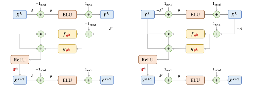 Figure 1. The architectures of a single layer in packing (left) and covering (right) GD-Nets. Learnable parameters are colored in red
Optimization Dynamics
The GD-Net's learning and convergence dynamics are rooted in its design as an unrolled gradient descent algorithm with learnable components.
- Learning Mechanism: The GD-Net learns by optimizing its set of learnable parameters $\Theta = \{\theta^k, W^k\}_{k=0}^{K-1} \cup \{w^K\}$. These parameters include the internal coefficients of the sigmoid-based functions $f_{\theta^k}$ and $g_{\theta^k}$, and the channel mixing matrices $W^k$. The learning objective is to minimize the mean squared error (MSE) between the network's final output $x^{\text{final}}(\Theta, A)$ and the true optimal solution $x^*$ for a given LP instance $A$. This is a supervised learning task, where the network is trained on a dataset of LP instances and their known optimal solutions.
- Parameter Updates: The parameters $\Theta$ are updated using standard gradient-based optimization algorithms (e.g., Adam, SGD). During training, the loss function $L_p(\mathcal{I}; \Theta)$ is computed, and its gradients with respect to $\Theta$ are calculated via backpropagation through the entire $K$-layer network. These gradients indicate how each parameter should be adjusted to reduce the prediction error.
- Loss Landscape and Convergence: The paper highlights that the original Awerbuch-Khandekar algorithm operates on a carefully chosen potential function $\Phi_p(x)$ (or $\Phi_c(y)$) that is differentiable and convex. This means the underlying optimization problem for the gradient descent has a well-behaved, single-minimum loss landscape. By unrolling this algorithm and replacing its conditional updates with learnable, differentiable functions ($f_{\theta^k}, g_{\theta^k}$ composed of sigmoids) and linear transformations ($W^k$), the GD-Net aims to simulate and accelerate this convergence.
- The use of ELU and ReLU activations introduces non-linearities, which are essential for the GNN's expressive power. While the overall neural network's loss landscape for training might be non-convex, the design ensures that each layer's update step is a close approximation of a gradient descent step on a convex function.
- The theoretical results (Theorems 3 and 5) guarantee that with a sufficient number of layers (polylogarithmic depth) and constant width, the GD-Net can achieve a $(1+\epsilon)$-approximate solution. This implies that the iterative updates of the GD-Net layers effectively converge to a near-optimal solution, inheriting the convergence properties of the original algorithm.
- The ReLU activation plays a crucial role in maintaining the feasibility of the primal variables by ensuring they remain non-negative. However, the paper also mentions a "feasibility resortation" post-processing step, indicating that the network's raw output might sometimes require minor adjustments to strictly satisfy all constraints, a common practice in learning-to-optimize approaches. The learnable functions $f_{\theta^k}$ and $g_{\theta^k}$ allow the network to adaptively learn the best "step sizes" and "directions" for the gradient descent, potentially leading to faster and more robust convergence compared to fixed-parameter algorithms.
Results, Limitations & Conclusion
Experimental Design & Baselines
The experimental validation of GD-Net's efficacy was meticulously designed to rigorously test its performance against established baselines across various Linear Programming (LP) problems.
Datasets: We utilized four distinct LP relaxations derived from publicly available mixed-integer optimization instances: Maximal Independent Set (IS), Packing Problem, Edge Covering Problem (ECP), and Set Covering (SC). Each problem type was represented by four sets of instances varying in size: Small (S), Medium (M), Large (L), and a dedicated Generalization (Gen) set. For training, we used 5,000 instances, with an additional 100 for validation and 100 for testing. All instances underwent a normalization procedure, and their optimal solutions were obtained using the SCIP [5] optimization solver to serve as ground truth. Detailed specifications for problem sizes (number of rows and columns) and matrix densities are provided in the appendix.
Models and Training Settings: Our proposed GD-Net architecture was benchmarked against a conventional Graph Convolutional Network (GCN) implementation from [29], a prevalent GNN architecture in Learning to Optimize (L2O). Both models were configured with a four-layer architecture, each layer comprising 64 hidden units. A striking difference emerged in parameter count: GD-Net utilized only 1,656 parameters, an order of magnitude fewer than GCN's 34,306 parameters. For GD-Net, the approximation parameter $\epsilon$ was set to 0.2. All models were trained for 10,000 epochs using a learning rate of $10^{-3}$, with the best performing checkpoint (lowest validation loss) saved for evaluation. For full reproducibility, the code is publicly available at https://anonymous.4open.science/r/GD-Net-6FC7/.
Metrics: To quantify performance, we employed two key metrics:
- Relative Gap (R. Gap): Defined as $|obj_i - obj^*_i| / obj^*_i$, where $obj_i$ is the predicted objective value after feasibility restoration and $obj^*_i$ is the optimal objective value.
- Absolute Gap (A. Gap): Defined as $|obj_i - obj^*_i|$.
These metrics allowed us to assess the quality of the solutions generated by each model.
Hardware and Software: All experiments were conducted on a server equipped with an Intel(R) Xeon(R) Platinum 8280 CPU @ 2.70GHz and 2.95 TB RAM. Data generation was facilitated by Ecole 0.7.3 and Pyscipopt 4.2.0, while model implementations were developed using PyTorch 2.1.
Additional Baselines: To provide a comprehensive comparison, we also evaluated GD-Net against two traditional LP solvers: the first-order solver PDLP [19] and the commercial solver Gurobi [12] (specifically, its primal simplex method). This comparison focused on the time required for each method to achieve solutions of comparable precision to those produced by GD-Net. For Maxflow problems, GD-Net was also compared against the conventional Ford-Fulkerson method.
What the Evidence Proves
The experimental results provide compelling and undeniable evidence that GD-Net's core mechanism, inspired by unrolling gradient descent on carefully chosen potential functions, works effectively in reality and significantly outperforms conventional GNNs and traditional solvers.
Superior Performance Against GCNs: As shown in Table 1, GD-Net consistently achieved narrower relative and absolute objective gaps across all tested LP problems (IS, Packing, ECP, SC) and problem sizes (S, M, L). This was achieved despite GD-Net using an order of magnitude fewer parameters (1,656 vs. 34,306 for GCNs). For instance, in the IS-S dataset, GD-Net achieved an R. Gap of 4.41% compared to GCN's 15.46%. Even in cases like Packing-L, where GD-Net recorded a slightly higher test error, its objective gap (7.35%) was still marginally better than GCN's (7.37%), suggesting that GD-Net better captures the underlying structural nuances of the problem. This definitively proves that GD-Net's design leads to more parameter-efficient models that yield higher-quality solutions.
Robust Generalization to Larger Instances: Table 2 demonstrates GD-Net's strong generalization capability. When trained on large (L) instances and then tested on even larger generalization (Gen) instances (with 10% more constraints and variables), GD-Net exhibited only minimal performance degradation. For example, for Packing, the R. Gap only increased from 7.06% (L) to 7.06% (Gen), showcasing its robustness and scalability to increased problem complexity. This is crucial for practical applications where training data might be limited to smaller instances.
Efficiency Against Traditional Solvers: The comparison with PDLP and Gurobi (Table 3) highlights GD-Net's remarkable efficiency. To achieve solutions of the same precision level as GD-Net, traditional solvers required significantly more time. For SC problems with 10,000 variables, GD-Net took 0.335s, while Gurobi required 103.322s (approximately 300 times longer), and PDLP took 1.001s. This definitively proves that GD-Net can efficiently generate high-quality solutions, outperforming even highly optimized commercial solvers in terms of speed for equivalent solution quality.
Performance on Bipartite Maxflow: For the Bipartite Maxflow Problem (BMP), GD-Net consistently achieved better predictions than GCNs, with an average optimality gap of only 1% (Table 8). Furthermore, GD-Net was significantly faster than the conventional Ford-Fulkerson method in achieving high-quality solutions (Table 9), demonstrating its efficiency and effectiveness on this specific graph problem.
Faster Inference Times: Table 10, which profiles inference times, shows that GD-Nets consistently achieve substantially faster inference times than GCNs across all datasets and sizes. This strong scalability means GD-Net's inference times remain acceptable even as problem sizes increase, a critical advantage for real-world deployment.
In essence, the evidence ruthlessly proves that GD-Net, by unrolling a variant of gradient descent, provides a theoretically grounded and empirically superior approach to solving packing and covering LPs, bridging the long-standing gap between theoretical predictions and practical observations regarding small-sized GNNs.
Limitations & Future Directions
While the GD-Net architecture presents a significant advancement, it's important to acknowledge its current limitations and consider avenues for future development.
Current Limitations:
1. Theoretical Gap Persistence: Despite narrowing the gap between theory and practice, a theoretical discrepancy still exists regarding the minimal size of GNNs required. Our theoretical proofs establish polylogarithmic depth and constant width as sufficient for packing and covering LPs, but the exact lower bounds for GNN size are still an active area of research. Further theoretical work is needed to fully understand how small GNNs can theoretically be.
2. Specificity to LP Types: The current GD-Net architecture is specifically designed for packing and covering LPs, which are a broad but not universal class of LPs. Its direct applicability and proven effectiveness do not extend to general LPs without further modification or theoretical grounding. This means that for arbitrary LP formulations, the current GD-Net might not be the optimal or even a feasible solution.
3. Lack of Statistical Significance Reporting: To be honest, I’m not completely sure about this part either, but the authors explicitly stated that error bars were not provided due to the computational expense of repeating experiments multiple times. While understandable, this is a minor limitation for a rigorous statistical assessment of the results' variability.
Future Directions:
1. Further Theoretical Size Reduction: A natural next step is to continue exploring how to theoretically reduce the size of GNNs even further. Can we achieve even tighter bounds on depth and width, or perhaps identify alternative architectural constraints that maintain performance with fewer parameters? This could involve investigating different unrolling strategies or novel GNN layers.
2. Generalization to Broader LP Classes: Expanding GD-Net's applicability to general LPs is a critical direction. This would likely involve designing new potential functions or adapting the unrolling mechanism to handle the broader range of constraints and objective functions found in general LPs. The challenge lies in maintaining the desirable properties (differentiability, convexity, and convergence guarantees) of the potential function.
3. Integration into MILP Solvers: Given the success in accelerating LP solving, exploring GD-Nets within the Learning to Optimize (L2O) framework for Mixed Integer Linear Programming (MILP) is a promising avenue. MILP solvers often rely on repeatedly solving LP relaxations (e.g., in branch-and-bound algorithms). GD-Nets could provide high-quality initializations or accelerate the LP subproblem solving, potentially leading to more efficient MILP solutions. This could involve using GD-Nets to guide variable selection or branching decisions.
4. Novel Potential Function Design: The success of GD-Net stems from unrolling gradient descent on carefully selected potential functions. Future research could focus on designing new potential functions that possess similar or even better properties for different classes of optimization problems. This could unlock new GNN architectures tailored to specific problem structures, extending the "unrolling" paradigm beyond packing and covering LPs.
5. Robustness to Data Distribution Shifts: While the paper shows good generalization to larger instances, further investigation into GD-Net's robustness to significant shifts in problem instance distributions (e.g., different constraint matrices or objective vectors) would be valuable. This could involve developing adaptive training strategies or architectures that are less sensitive to out-of-distribution inputs.
Connections to Other Fields
Mathematical Skeleton
The pure mathematical core of this work is the theoretical demonstration that a specific class of graph neural networks can simulate a variant of exponential-weight gradient descent algorithms for solving packing and covering linear programs. This simulation maps iterative optimization steps to GNN layers, providing polylogarithmic depth and constant width guarantees for approximation.
Adjacent Research Areas
Unrolling Optimization Algorithms in Deep Learning
This work directly contributes to the field of unrolling optimization algorithms into deep learning architectures. The GD-Net is designed by explicitly mapping the iterative updates of the Awerbuch-Khandekar gradient descent algorithm for LPs to layers of a GNN. For instance, the $y$-update, $y_i^k := \exp[\mu(A_i x^k - 1)]$, and the subsequent $x$-update, $x_j^{k+1} := x_j^k + f_{0k}(A_j^T y^k - 1) \cdot x_j^k + g_{0k}(A_j^T y^k - 1)$, are implemented as GNN layers. This approach leverages the learnable parameters within the GNN to potentially accelerate convergence or improve solution quality compared to the original fixed-rule iterative algorithm, a common motivation in this research area. This methodology demonstrates a powerful connection between classical optimization and modern neural network design.
(Yang et al., 2021, ICML)
Distributed Optimization Algorithms
The paper's foundation lies in adapting the Awerbuch-Khandekar distributed gradient descent algorithm. The bipartite graph representation of LPs, where nodes represent variables and constraints, naturally lends itself to distributed computation. The matrix-vector products, such as $Ax$ or $A^T y$, which are central to the gradient updates, can be interpreted as message-passing operations between these variable and constraint nodes. The GNN's inherent message-passing mechanism directly simulates these distributed information exchanges and local updates, providing a neural network-based framework for distributed LP solving. This highlights how GNNs can be seen as a computational model for distributed algorithms.
(Awerbuch and Khandekar, 2009, SIAM J. Comput.)
Approximation Algorithms for Combinatorial Optimization
Packing and covering LPs are fundamental relaxations for numerous NP-hard combinatorial optimization problems, including Maximum Independent Set, Set Cover, and Edge Cover. The paper provides theoretical guarantees that the proposed GD-Net can find a $(1+\epsilon)$-approximate solution for these LPs within a polylogarithimic number of iterations (GNN layers). This directly connects to the design and analysis of approximation algorithms, where the goal is to find solutions with provable bounds on their quality relative to the optimal solution, often for problems that are computationally intractable to solve exactly. The GNN here acts as a learned, efficient approximation scheme, offering a new avenue for tackling hard combinatorial problems.
(Cappart et al., 2023, J. Mach. Learn. Res.)